HOW TO USE ARRAYFORMULA FUNCTION IN GOOGLE SHEETS ?

INTRODUCTION

ARRAYFORMULA is one of the very powerful and useful formulae in GOOGLE SHEETS which can be used as a master key to work perfectly by extending the limits of the simple functions in google sheets.

An ARRAYFORMULA FUNCTION allows simple functions to return the result as ARRAY FUNCTION which can extend the result to multiple rows and columns.

ARRAYFORMULA FUNCTION HELPS US TO GET THE RESULT FROM THE ARRAY FORMULAS AND USE OF NON ARRAY FORMULAS TO BEHAVE LIKE ONE. WE CAN USE SIMPLE NON ARRAY FUNCTIONS LIKE THE ARRAY FORMULAS AS WE’LL DISCUSS FURTHER IN THE EXAMPLES.

The possibilities with this function becomes endless. The requirement of array formulas is fulfilled with this general function which can be used almost anywhere to completely automate the outcome of the functions.

In this article we would learn about the purpose, syntax, formula of the ARRAYFORMULA and get a better understanding with the help of the examples in GOOGLE SHEETS .

PURPOSE OF ARRAYFORMULA FUNCTION IN GOOGLE SHEETS

ARRAYFORMULA SIMPLY ENABLES THE FUNCTIONS TO RETURN THE RESULTS IN MULTIPLE ROWS OR COLUMNS. IT MAKES THE NON ARRAY FUNCTION TO BE ABLE TO RETURN THE RESULT AS AN ARRAY FUNCTION.

For example,

Suppose, we have two parallel columns containing some random numbers and we want to find out the sum of individual rows.

i.e. the situation is somewhat like shown in the table below.

SERIES 1	SERIES 2	TOTAL
17	49	66
24	12	36
37	38	75
19	24	43
34	18	52
47	50	97
42	24	66
27	41	68
36	20	56
36	27	63
35	23	58
46	17	63

THE SERIES ARE SUMMED UP ACROSS

There can be a few solutions for this example.

1. Use the operator + and find out the sum in the first row. Drag down the function to find out all the results.
2. Find out the result individually for all the series, which is not recommended.
3. Use SUM function and then again drag down the function.

What if we want to perform this task in one go.

Well, that can only be done when a function has the ability to return an array and the basic operators or the SUM function doesn’t have that ability.

This is one of the situations, where we can make use of the ARRAYFORMULA and make the + operator perform the complete job in one go.

We’ll see this in action in the examples discussed below.

PREREQUISITES TO LEARN ARRAYFORMULA FUNCTION

THERE ARE A FEW PREREQUISITES WHICH WILL ENABLE YOU TO UNDERSTAND THIS FUNCTION IN A BETTER WAY.

•  Basic understanding of how to use a formula or function.
•  Basic understanding of rows and columns in GOOGLE SHEETS .
• Some information about the ARRAY FORMULAS.
•  Of course, availability of internet and google sheets login.
  
  
  

SYNTAX: ARRAYFORMULA FUNCTION

The Syntax for the RANDARRAY function is

=ARRAYFORMULA (EXPRESSION OR FUNCTION OR ARRAY FUNCTION )

EXPRESSION OR FUNCTION OR ARRAY FUNCTION is the expression consisting of the basic operators, or any function or the array function itself which return the single output or multiple line output (in Case of array functions )

EXAMPLES: ARRAYFORMULA FUNCTION IN GOOGLE SHEETS

EXAMPLE TYPE 1: USE ARRAYFORMULA TO SUM UP TWO SERIES USING EXPRESSION

TARGET : SUM TWO GIVEN SERIES OF NUMBERS HORIZONTALLY IN ONE STEP

This is the same example which we brought into our discussion earlier.

Let us again get the data.

SERIES 1	SERIES 2	TOTAL
17	49
24	12
37	38
19	24
34	18
47	50
42	24
27	41
36	20
36	27
35	23
46	17

We need to find out the result of the given two series using the ARRAYFORMULA function in one step.

The data in the google sheets is as shown in the picture below.

Follow the steps to sum up the numbers horizontally as required .

STEPS TO SUM THE SERIES HORIZONTALLY IN GOOGLE SHEETS

• Go to the result cell for first case i.e. E7
• Enter the formula as =ARRAYFORMULA(C7:C18+D7:D18).

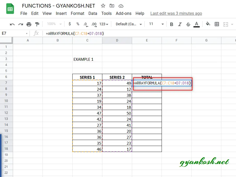
• Press ENTER.
• The google sheets will display the sum of the series 1 and series 2 as shown below.
  
  

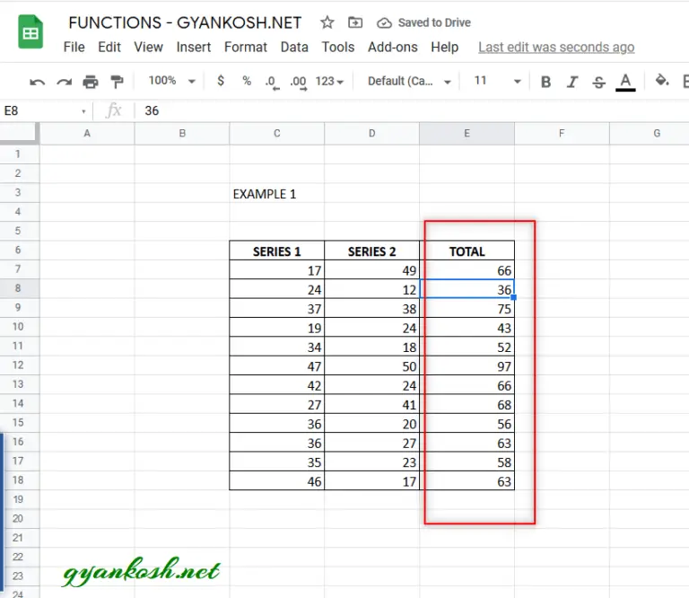
EXPLANATION:

In this example, we can see that a single formula performed all the task in one go which is only possible in the array functions.

If we didn’t use ARRAYFORMULA FUNCTION, we need to find out the individual sum and then use the drag function. If there are five series, we need five drag operations.

This method saved our time and resources.

EXAMPLE TYPE 2: USING ARRAYFORMULA FUNCTION WITH AN ARRAY FUNCTION

We already tried arrayformula function with an expression.

Now let us try this function with an array function.

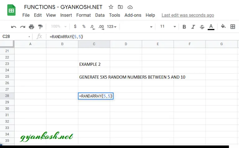
TARGET: GENERATE 5X5 GRID OF RANDOM NUMBERS BETWEEN 0 AND 10

SOLUTION:

We’ll go into the solution step wise step.

The first step is to find a function which will create a grid of random numbers for us.

RANDARRAY FUNCTION is the answer to this problem. The RANDARRAY FUNCTION will give us a grid of the desired size.

The next problem is that the

RANDARRAY FUNCTION will generate the numbers between 0 and 1.

We can multiply the numbers with 10, so that they’ll become between 0 and 10, but the problem is that, as soon as we multiply it with 10, it won’t behave as an array function but only a simple function and return only one number.

The next problem is that we need only the round numbers and not the decimal portion.

We can use many functions for that operation like INT or ROUND etc. but the problem is that as soon as we make use of those functions, the array function RANDARRAY won’t generate the grid but only one number. We’ll use INT function for this problem.

As we enter the function INT, the RANDARRAY FUNCTION is no more an array function but a simple non array function.

Now we have all the solutions but two problems with the multiplying factor 10 and the function INT.

Here we deploy our newly learnt function ARRAYFORMULA to help us get out of this situation.

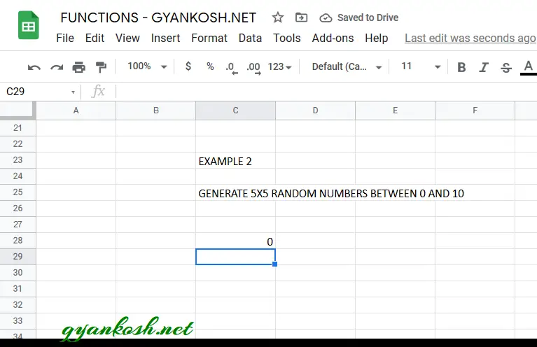
STEPS TO CREATE A GRID OF 5X5 NUMBERS BETWEEN 0 AND 10:

• Select the cell where we want the first number to show.
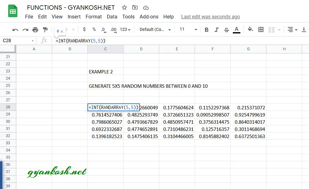
• Enter the formula as =ARRAYFORMULA(INT(RANDARRAY(5,5)*10))

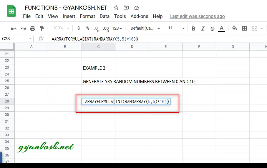
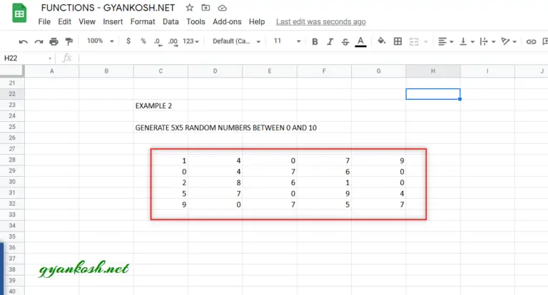
• Press ENTER.
• The result will appear as shown in the picture below.
• The EXPLANATION of the formula follow the picture.

EXPLANATION:

Let us understand the working of the formula.

We used the formula

=ARRAYFORMULA(INT(RANDARRAY(5,5)*10))

The first function used is the ARRAYFORMULA which lets us make the NON ARRAY FORMULAS AS ARRAY FORMULAS. In our expression INT function is a non array formula.

The INT function returns a whole number less than or equal to the NUMBER passed into INT.

For example =INT(15.12) will return 15 ,

=INT(89.98) will return 89 and so on.

RANDARRAY as we already discussed in previous example, will create the grid of 60 elements between 0 and 1 so we multiplied it with 50 which will return us the numbers between 0 and 10.

In this article we learnt the various ways of using ARRAYFORMULA in google sheets.