Table of Contents
- INTRODUCTION
- WHAT ARE ALTERNATE ROW COLORS IN GOOGLE SHEETS?
- PURPOSE OF ALTERNATE ROW COLORS IN GOOGLE SHEETS
- STEPS TO APPLY ALTERNATE ROW COLORS IN GOOGLE SHEETS
- USE ALTERNATE ROW COLORS USING MANUAL WAY
- PROS OF MANUAL WAY OF USING ALTERNATING COLORS
- CONS OF MANUAL WAY OF USING ALTERNATING COLORS
- ALTERNATING COLORS OPTION
- BUTTON LOCATION FOR ALTERNATING COLORS OPTIONS
- HOW TO REMOVE ALTERNATING COLORS FROM THE GIVEN ROWS
INTRODUCTION
GOOGLE SHEETS provide us with many ready to use functionalities which makes our working quite easier.
One of such points is the fonts and colors which lets us segregate the different classes of the data. In addition to this segregation or visual classification, colors and fonts are important because they make the data and values visible and more readable too.
The alternating colors help us to make the data more readable by giving the alternate rows different shades.
In this article, we’d learn to put alternate colors in google sheets.
WHAT ARE ALTERNATE ROW COLORS IN GOOGLE SHEETS?
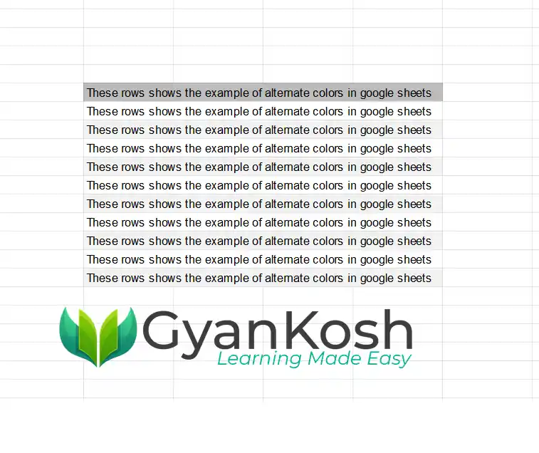
ALTERNATE ROW COLORS MEANS TO FILL THE BACKGROUND OF THE ALTERNATE ROWS WITH THE DIFFERENT SHADES TO MAKE THE DATA MORE PROMINENT AND READABLE.
The following picture shows the sample of alternate row colors.
PURPOSE OF ALTERNATE ROW COLORS IN GOOGLE SHEETS
The alternate row colors option provides us a few benefits for which we can opt these functions.
- It’ll make the text or data more readable.
- It’ll improve aesthetics.
- It’ll help us classify the data.
STEPS TO APPLY ALTERNATE ROW COLORS IN GOOGLE SHEETS
We can apply alternate row colors in google sheets in the following ways.
- MANUAL WAY
- ALTERNATE COLORS OPTION
USE ALTERNATE ROW COLORS USING MANUAL WAY
We can easily use alternate colors using the forced method.
Forced method is the one when we select the cells and choose the background colors.
FOLLOW THE STEPS TO USE ALTERNATE ROW COLORS MANUALLY
- Select one row of the cells where you want the shade or color.
- Go to FILL COLOR option and choose the color you want.
- After choosing the color, Select the next row.
- Go to FILL COLOR and choose the second shade.
- Repeat the process and fill the complete rows with the same shades.
PROS OF MANUAL WAY OF USING ALTERNATING COLORS
- You can choose any color of your choice.
- You can choose any difference or combination of the color shades.
- Any kind of variations can be opted.
- More than two shades can be chosen which is not possible otherwise.
CONS OF MANUAL WAY OF USING ALTERNATING COLORS
- The method is time consuming. Choosing every row and then coloring it will take much time. [ A bit faster method is shown below].
- Some users may find it difficult to choose the shades from the available options.
- If the data is too big, this method is impossible as choosing every line is tough and time consuming.
- There are chances of shade issue. Every time the user needs to choose the same shade. There can be a mistake which will further time consuming.
For all these issue, we can speed up the process a bit by using the following tip.
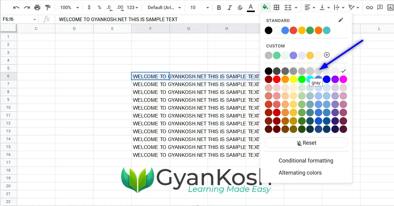
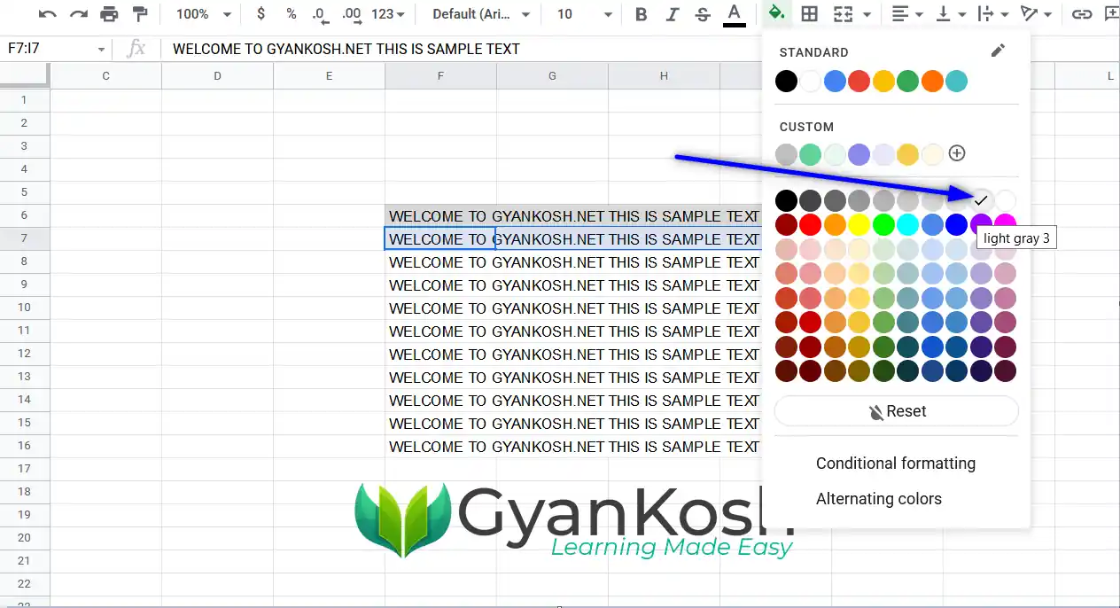
IF YOU ARE USING THE MANUAL WAY OF ADDING ALTERNATING COLORS IN THE ROWS, YOU CAN SELECT ALL THE ROWS BY KEEPING THE CONTROL KEY PRESSED, AND CLICKING ON ALL THE ROWS. THE SELECTION WILL KEEP ON ADDING. NOW SIMPLY SELECT ONE COLOR FROM THE FILL COLOR OPTION.
REPEAT THE PROCESS FOR THE SECOND SET OF ROWS.
Simply select all the rows and choose the color shade.
The following picture shows the process.

If we don’t have any issues or requirements which can be fulfilled only with the help of manual method, we should go for the dedicated option for alternating colors.
ALTERNATING COLORS OPTION
This is a dedicated option which help us to put alternating colors in the rows within seconds for any size of the data.
BUTTON LOCATION FOR ALTERNATING COLORS OPTIONS
The alternating color option is present under the FORMAT MENU > ALTERNATING COLORS.
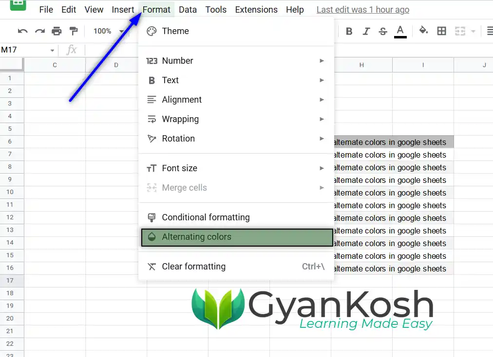
Let us learn to use ALTERNATING COLORS option to put shades in the alternating rows.
FOLLOW THE STEPS TO USE ALTERNATING COLORS OPTION
- Select all the cells or rows where you want to put the alternating colors.

- Go to FORMAT MENU and choose ALTERNATING COLORS.
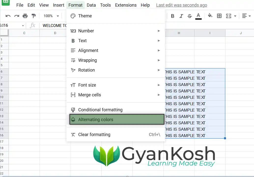
As we choose ALTERNATING COLORS, the option will open on the right portion of the screen.
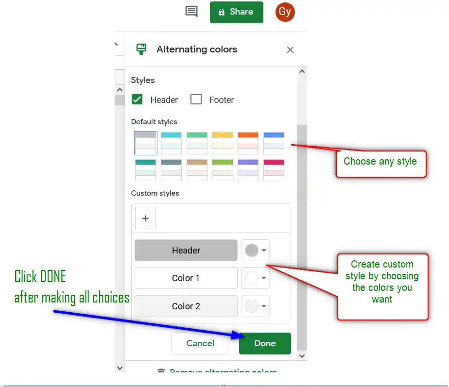
THE EFFECTS OF THE SETTINGS OPTIONS ARE AS FOLLOWS.
| OPTION | DETAILS |
| STYLES | CHOOSE HEADER OR FOOTER IF THERE IS ONE. ITLL GIVE IT A DARK COLOR |
| DEFAULT STYLES | CHOOSE STYLES FROM THE READY TO USE OPTIONSCH |
| CUSTOM STYLES | CHOOSE THE COLORS OF YOUR CHOICE. CREATE CUSTOM STYLES. |
- For our example, we chose a default style as shown in the picture below.
- Click DONE.
As we click DONE, alternating colors will be applied to the selected cells.
The following picture shows the results.
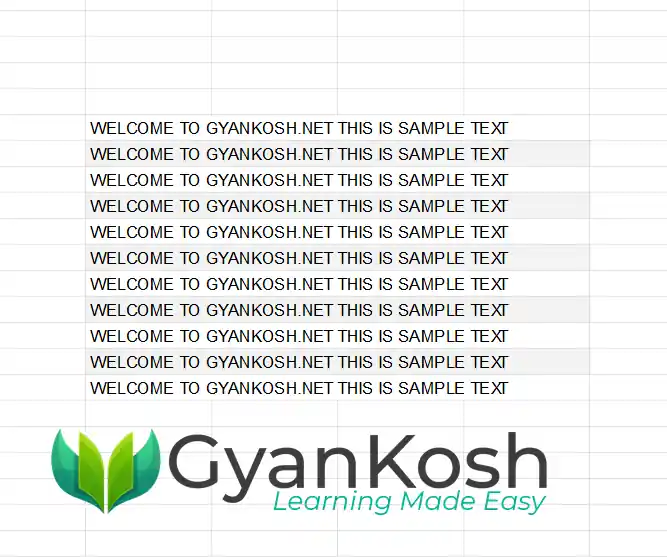
In these ways, we can create alternating colors.
HOW TO REMOVE ALTERNATING COLORS FROM THE GIVEN ROWS
If we want to remove the alternating colors from the given rows., simply removing the color from the rows might not be enough.
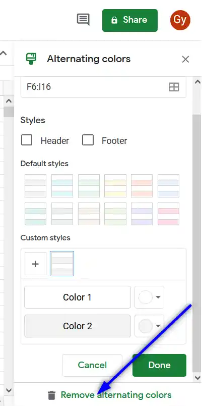
FOLLOW THE STEPS TO REMOVE THE ALTERNATING COLORS FROM THE GIVEN ROWS OR CELLS
- Click anywhere in the alternating colors group.
- Go to FORMAT MENU> ALTERNATING COLORS.
- It’ll open the options on the right.
- Click REMOVE ALTERNATING COLORS option which is present at the bottom.
- The alternating colors will be removed.