INTRODUCTION
“MERGING IS THE PROCESS OF JOINING THE TWO OR MORE CELL IN GOOGLE SHEETS”.
THE CELLS CAN BE IN SAME ROW OR DIFFERENT ROWS. THE CELLS CAN BE IN ROWS OR COLUMNS BUT NEED TO BE ADJACENT.
WHEN TO USE MERGE IN GOOGLE SHEETS?
As the name suggests it does the job of merging (join the two cells into one) two cells.
The two cells are merged for the presentation purpose mainly, or if there is a group which belong to the same class or any particular need as per choice.
It is also done when we have a class and there are many sub classes which we want to show under a main Class.
If we don’t want to use WRAP TEXT merging can be done to make the cells longer.
EXAMPLE OF MERGE TEXT IN GOOGLE SHEETS
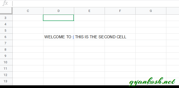
Just take a look at the picture below.
It is clearly visible in the above picture, that the content of the cell 1 is hidden and the content of the cell 2 started from the second cell. The complete text “Welcome to Gyankosh” is not visible in the cell. Hello is the content of other cell. This kind of cases can be tackled with the help of Wrap Text as well as by merging cells.
Wrap text would broaden the cell whereas Merging the text would give it more space.
Another apt situation for using the MERGE option in Google Sheets is when we are preparing any report comprising of the sub sections or classification.
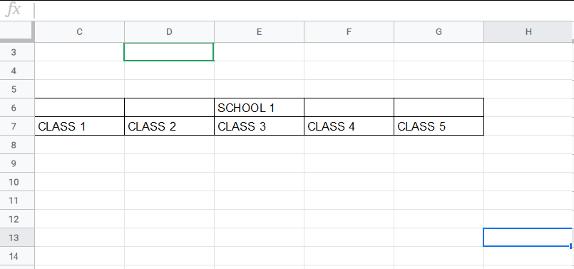
Look at the picture below.
In the picture above , the school is showing five classes.
Although any intelligent person can tell that All the classes are under School 1 but School1 is above CLASS 3 only, which can create a confusion. [ It is just for an example. There can be reports which can create very serious problems if the classification is not shown properly ].
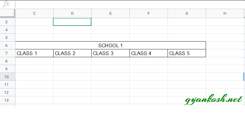
If we want to show the school 1 above all the five classes, we can use the MERGE option and the table would become as shown in the picture below. The second table using the MERGE option looks better and more informative.
So let us find out how we can use the MERGE option in google sheets to solve these problems.
STEPS TO MERGE CELLS IN GOOGLE SHEETS
- Select the cell/cells where the MERGING needs to be done.
- CLICK on the button MERGE CELLS BUTTON.
- The result is visible as shown in the picture.
- The complete text is shown in the cell by merging all the selected cells into one. [ The data of the UPPER LEFT cell will be kept. Rest will be removed ]
OTHER OPTIONS TO MERGE CELLS IN GOOGLE SHEETS
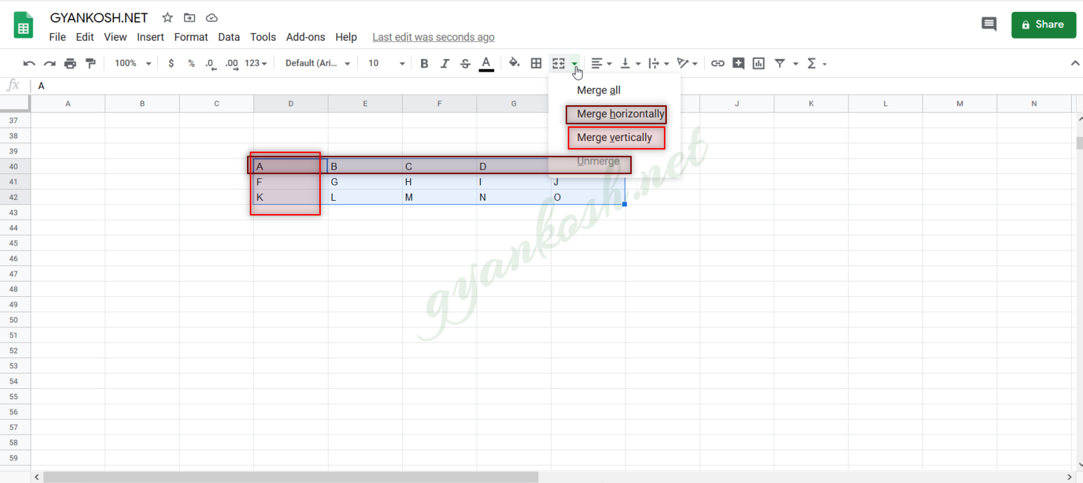
In addition to the above mentioned option of merging, few more options are present in the menu, which will be shown if the down arrow near the button is clicked. The pic is shown in the following picture.
MERGE HORIZONTALLY
MERGE VERTICALLY:
UNMERGE CELLS:
MERGE THE CELLS HORIZONTALLY. ALL THE COLUMNS WILL BE MERGED BUT ROWS WON’T BE MERGED.
MERGE THE CELLS VERTICALLY. ROWS WILL BE MERGED BUT COLUMNS WON’T BE MERGED.
REMOVE ALL THE MERGING FROM THE SELECTED CELLS.
ANIMATED EXAMPLE OF MERGING CELLS IN GOOGLE SHEETS
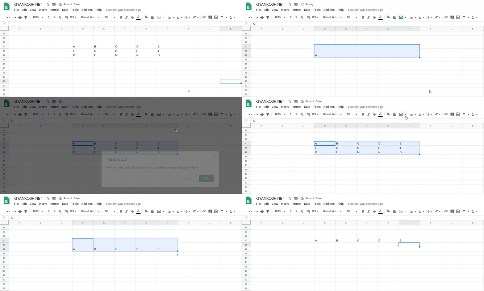
EXPLANATION:
MERGE HORIZONTALLY:
Let us learn how can we merge the cells horizontally.
The picture above shows the process of merging the cells horizontally.
Select all the cells and click on the dropdown arrow of MERGE CELLS button as shown in the picture above. Choose MERGE HORIZONTALLY.
It’ll merge the columns of the row.
MERGE VERTICALLY:
Let us learn how can we merge the cells vertically .
The picture above shows the process of merging the cells vertically.
Select all the cells and click on the drop down arrow of MERGE CELLS
button as shown in the picture above. Choose MERGE HORIZONTALLY.
It’ll merge the columns of the row.
UNMERGE CELLS:
Select all the merged cells and go to MERGE CELLS DROPDOWN and choose UNMERGE. It’ll remove all the merging.
