Table of Contents
- INTRODUCTION
- WHY TO USE HYPERLINKS IN GOOGLE SHEETS
- DIFFERENT WAYS TO INSERT HYPERLINKS IN GOOGLE SHEETS
- METHOD 1 : CREATING DIRECT HYPERLINK IN GOOGLE SHEETS
- METHOD 2 : CREATING HYPERLINK USING A MENU OR TOOLBAR OPTION IN GOOGLE SHEETS
- METHOD 3 : CREATING HYPERLINK USING THE HYPERLINK FUNCTION IN GOOGLE SHEETS
INTRODUCTION
When we are using any reports, we might need to go different locations in the workbook, or any website, or open a different format file and so on. For such situations, we use the functionality called HYPERLINKS.
We need to create and use hyperlinks very often in the sheets we create.
“HYPERLINK” IS A TEXT OR ANY LINK WHICH WILL TAKE THE USER TO THAT PARTICULAR LOCATION AFTER CLICKING IT. THE LOCATION CAN BE A SHEET IN THE SAME WORKBOOK, ANOTHER WORKBOOK, ANY WEBSITE, ANY CONTENT WHICH.
The hyperlinks can be inserted in different ways such as using the OPTION FOR INSERTING HYPERLINK or using a HYPERLINK FUNCTION.
In this article we will learn to insert a hyperlink and link different address or contents using the two methods mentioned
WHY TO USE HYPERLINKS IN GOOGLE SHEETS
The HYPERLINKS or the we call them MAGIC TEXT are very useful when we want to give our user a perfect and easy experience while using the report or any presentation or any document.
There can be a number of situations and reasons to use them. A few are following.
Hyperlinks are used when
- We want our users to REACH ANY ADDRESS DIRECTLY WITHOUT ANY MISTAKE.
- We want the user to reach a website directly and not bother about typing of pasting any website address.
- When we want to give our link a BETTER WORD to describe about the target link or location.
- We want to save the time of the users.
DIFFERENT WAYS TO INSERT HYPERLINKS IN GOOGLE SHEETS
GOOGLE SHEETS provide us many ways to insert the hyperlinks in google sheets.
We’ll discuss all the ways in detail.
The following methods can be used to insert a hyperlink in google sheets.
- CREATING DIRECT HYPERLINK
- USING THE MENU OR TOOLBAR OPTION
- USING FUNCTION
METHOD 1 : CREATING DIRECT HYPERLINK IN GOOGLE SHEETS
Google Sheets is a pro when it comes to connectivity. It is so lively about the links and various other options.
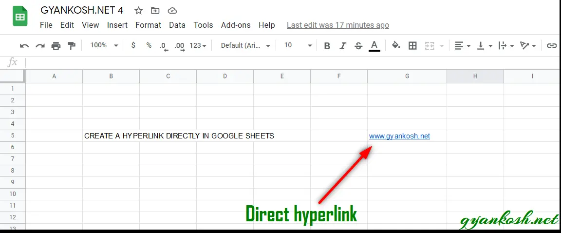
IF WE DIRECTLY TYPE ANY LINK IN GOOGLE SHEETS, IT’LL BECOME A HYPERLINK ITSELF WITH THE SAME LABEL. E.G. IF WE TYPE WWW.GYANKOSH.NET , IT’LL CREATE A HYPERLINK WITH A TEXT “WWW.GYANKOSH.NET” POINTING TO THE SAME WEBSITE I.E. WWW.GYANKOSH.NET
Let us take an example of the same.
FOLLOW THE STEPS TO INSERT A DIRECT HYPERLINK IN GOOGLE SHEETS.
- Select the cell where you want to insert the hyperlink.
- Type in the link directly in the cell.
- Click Enter.
- The hyperlink is ready.
You can use the hyperlink by simply clicking this text.
METHOD 2 : CREATING HYPERLINK USING A MENU OR TOOLBAR OPTION IN GOOGLE SHEETS
We inserted a link directly but we can’t change the TEXT LABEL in this method.
So, we can opt for other methods to create a hyperlink with a different label.
THERE ARE OPTIONS TO INSERT THE LINKS AVAILABLE IN MENU AS WELL AS DIRECT ACCESS IN THE TOOLBAR.
Let us understand this using an example.
FOLLOW THE STEPS TO INSERT A HYPERLINK USING MENU OPTION OR TOOLBAR OPTION IN GOOGLE SHEETS.
- Select the cell where you want to insert the hyperlink.
- Go to INSERT MENU and choose INSERT LINK as shown in the picture below.
You can use the hyperlink by simply clicking this text.

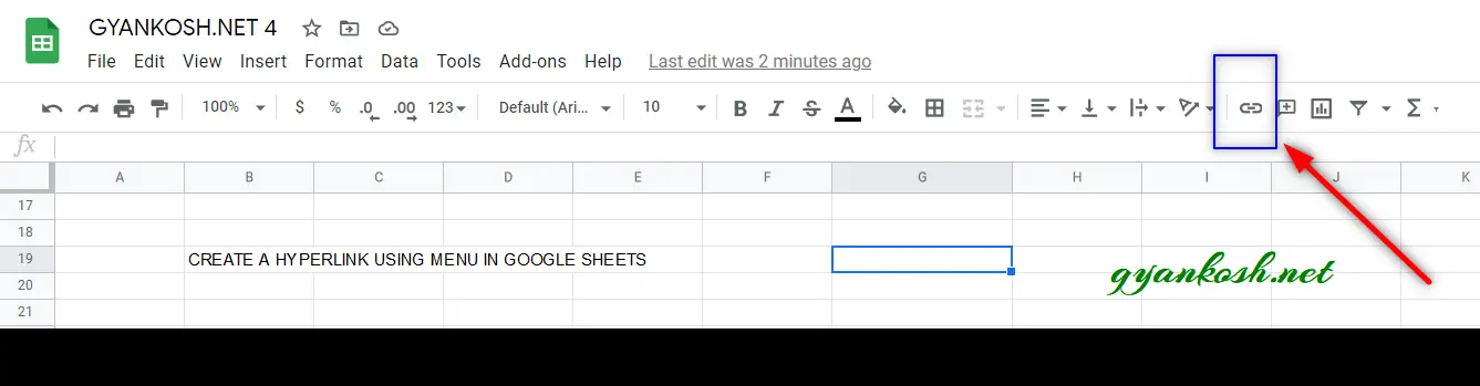
The same option is available on the toolbar also. We can choose that option too.
The following picture shows the location of the INSERT LINK button on the toolbar.
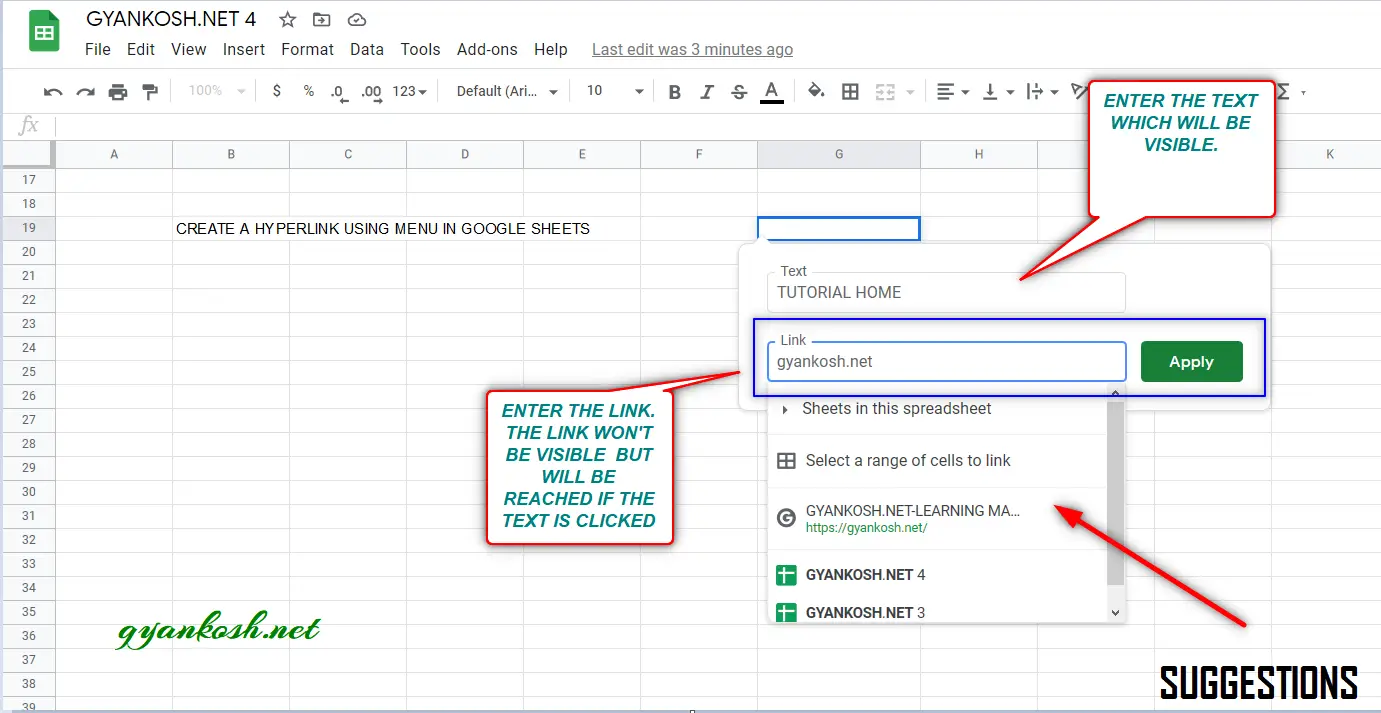
After clicking the option to INSERT LINK from the menu or the toolbar , a small window will open adjacent to the selected cell.
The window will have the two fields.Enter the LABEL or the FACE TEXT in the TEXT FIELD as shown in the picture below.
This will be the visible text.
Now, enter the link or url in the LINK FIELD as shown in the picture below. It’ll be the target link which will be fired when the TEXT or LABEL is clicked.
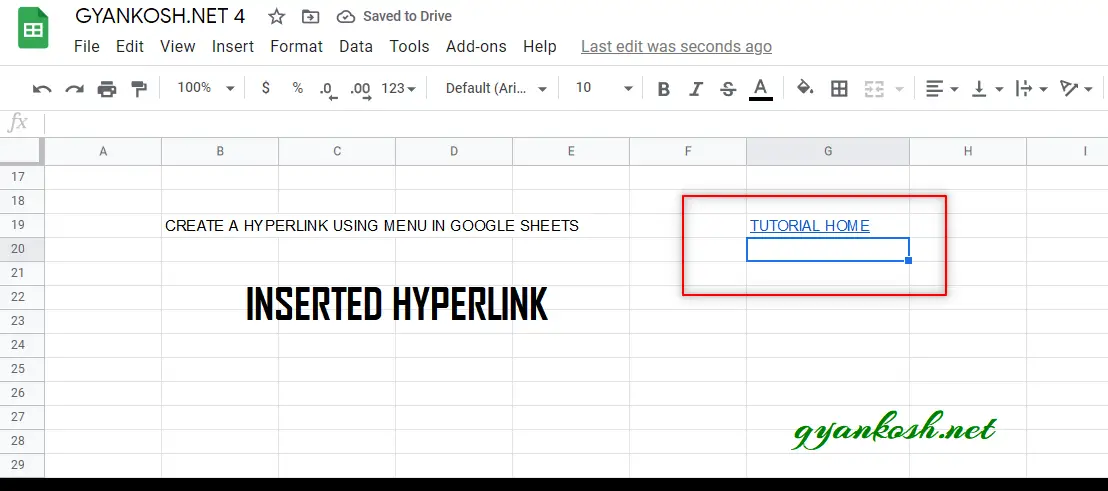
After entering the desired TEXT or LABEL and the target link, press ENTER.
The TEXT will be visible in the Cell and the link will be hidden as shown in the picture below.
When we click the Hyperlink [ Text which we just entered and stuck to the link ] , the Google Sheets will take us to the address.
The following picture shows the inserted hyperlink.
The same option is available on the toolbar also. We can choose that option too.
The following picture shows the location of the INSERT LINK button on the toolbar.
The same option is available on the toolbar also. We can choose that option too.
The following picture shows the location of the INSERT LINK button on the toolbar.
The same option is available on the toolbar also. We can choose that option too.
The following picture shows the location of the INSERT LINK button on the toolbar.
METHOD 3 : CREATING HYPERLINK USING THE HYPERLINK FUNCTION IN GOOGLE SHEETS
We can also insert the HYPERLINK using a function which is named the same i.e. HYPERLINK FUNCTION.
The SYNTAX of the HYPERLINK FUNCTION
=HYPERLINK ( ” URL / ADDRESS “, ” TEXT or LABEL “)
URL Link of the target.
TEXT The label to be used.
Let us take an example to learn the same.
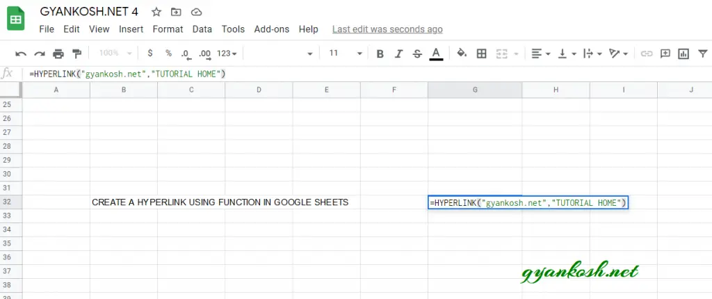
Let the url be gyankosh.net and the Text be TUTORIAL HOME.
FOLLOW THE STEPS TO INSERT HYPERLINK USING THE FUNCTION IN GOOGLE SHEETS
- Select the cell where you want to insert the hyperlink.
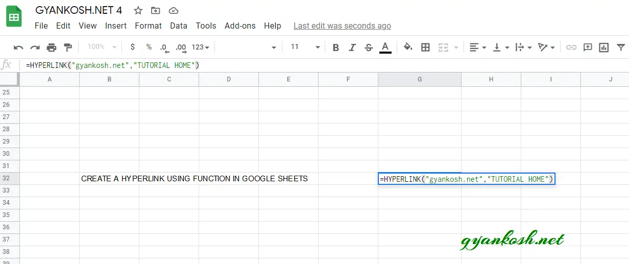
- Enter the formula as =HYPERLINK (“gyankosh.net”,”TUTORIAL HOME”) and press Enter.
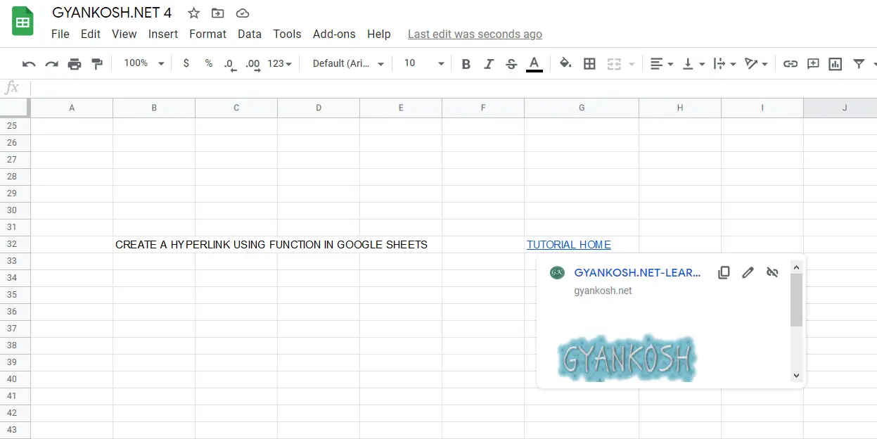
- The Hyperlink bearing the text TUTORIAL HOME will be inserted in the google sheet.
Following picture shows the created hyperlink using function in google sheets.

In this article we learned about the creation of hyperlinks using different methods.