INTRODUCTION
So , we have discussed the different ways to INSERT EURO SYMBOL IN GOOGLE SHEETS. But what about the situation when we are creating any Accounting report and we need to format the cells to show the EURO SYMBOL in front of every number which can be denoted as a currency.
As we know the spreadsheets are used by accounting people a lot. There is always a provision of using the currency symbols separately and so is found in the google sheets to.
In this article, we’ll learn to format our cells such that a EURO SYMBOL is visible before every number or figure entered.
WHY WE NEED FORMATTING AS EURO SYMBOLS
Inserting the EURO symbols in front of numbers or currency
such as
€ 45 + €67 = €112
This type of calculations are more informative and the nicest thing about them is that they never interfere with our calculations yet they stick to the number.
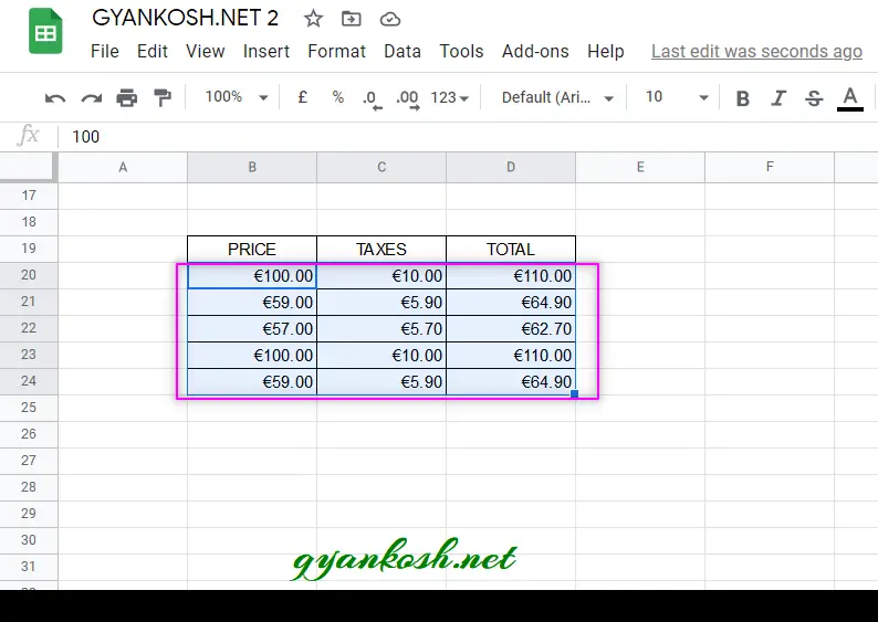
A small sample of calculation is shown below which is created in the google sheets only.
| PRICE | TAXES | TOTAL |
| €100.00 | €10.00 | €110.00 |
| €59.00 | €5.90 | €64.90 |
| €57.00 | €5.70 | €62.70 |
| €100.00 | €10.00 | €110.00 |
| €59.00 | €5.90 | €64.90 |
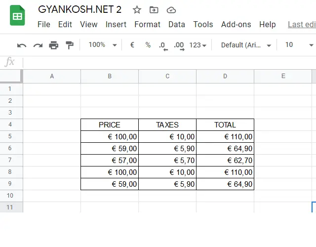
The table shows a EURO SIGN against every figure, but we haven’t inserted it using the other procedures but just formatted our cells to show the currency symbol.
We’ll learn the method further in the same article.
STEPS TO FORMAT THE CELLS TO SHOW EURO SYMBOL BEFORE EVERY NUMBER
There are two options of formatting the cell for EURO CURRENCY FORMAT.
- Setting the LOCALE and using FORMAT AS CURRENCY BUTTON.
- Using CURRENCY FORMATS to set the format for EURO CURRENCY.
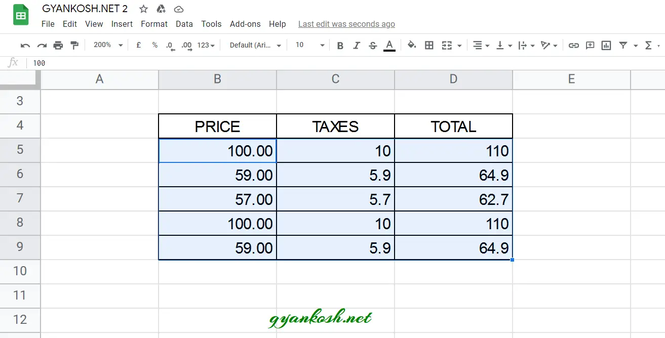
Let us take an example to apply EURO BEFORE NUMBER in the following cells.
The table contains price, taxes and total amount but we haven’t applied any currency format in the cells.
Now , let us try to apply the EURO symbol before every cell.
| PRICE | TAXES | TOTAL |
| 100.00 | 10 | 110 |
| 59.00 | 5.9 | 64.9 |
| 57.00 | 5.7 | 62.7 |
| 100.00 | 10 | 110 |
| 59.00 | 5.9 | 64.9 |
Follow the steps to apply EURO SYMBOL in front of every cell.
Select the cells where we want to apply the EURO CURRENCY FORMAT.
2. USING CURRENCY FORMAT TO FORMAT THE CELLS FOR EURO SYMBOL
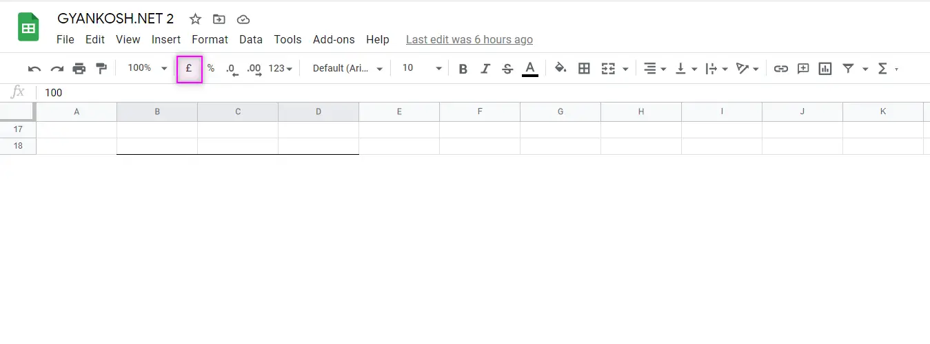
The Currency Format Button is located in the Toolbar itself as shown in the picture below.
THE FORMAT AS CURRENCY BUTTON WILL FORMAT THE SELECTED CELLS INTO CURRENCY FORMAT IMMEDIATELY AS PER THE LOCALE SELECTED.
The following picture shows the button location for FORMAT AS CURRENCY option.
FOLLOW THE STEPS TO SET THE FORMAT AS CURRENCY OPTION [ EURO ]:
- Select the cells which you want to format as CURRENCY EURO.
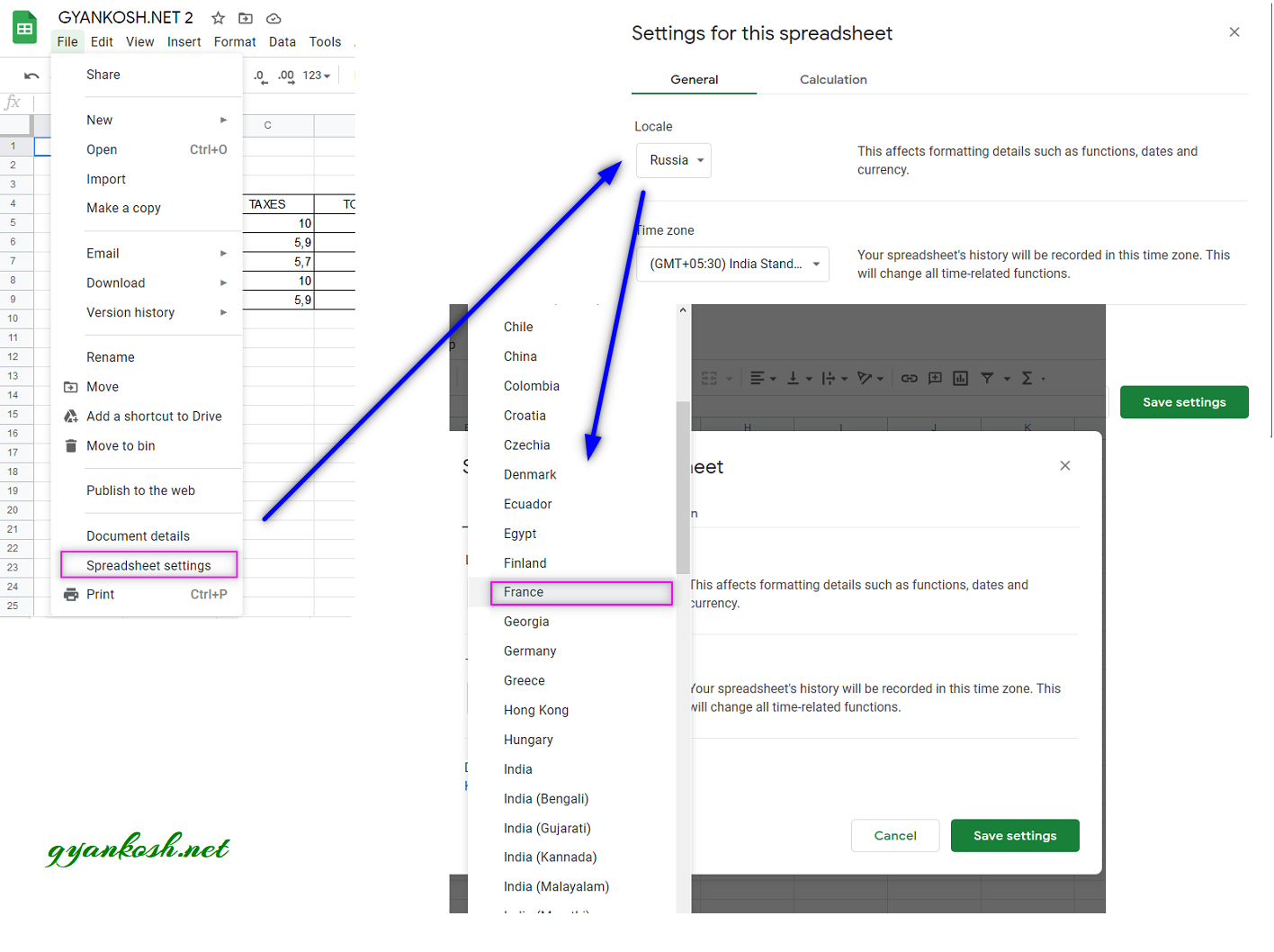
- Go to FILE MENU and choose SPREADSHEET SETTINGS.
- A small window will open asking for the LOCALE.
- Choose the locale as the country whose currency you want to use. [ For this case we can use ITALY or any other European country which has EURO as currency.
- Press SAVE SETTINGS.
- The process is shown in the picture below.
- After choosing the country [ locale] , the following screen will be visible.

- Click SAVE SETTINGS.
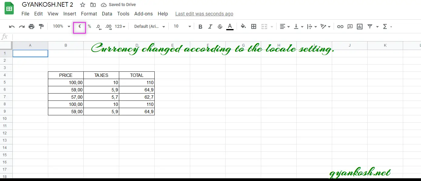
- The FORMAT AS CURRENCY button will change to the currency of the LOCALE SELECTED.
- After selecting ITALY, the format as currency button will change to EURO as shown in the picture below.
- Now select all the cells where we want to change the format as EURO CURRENCY.
- Simply Click the FORMAT AS CURRENCY button as shown in the picture below.
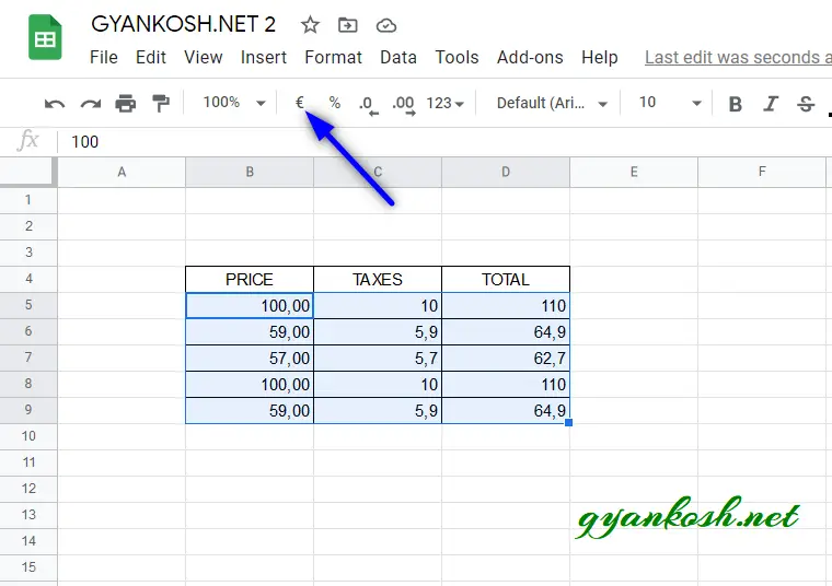
A EURO symbol will be applied in front of all the numbers in the selected cells.
The following picture shows the result.
2.FORMAT THE CELLS AS EURO CURRENCY USING MORE FORMATS
If we want to use the currency format randomly and don’t want to change the locale, this method can be used easily.
FOLLOW THE STEPS TO CHANGE THE FORMAT OF THE CELLS TO EURO CURRENCY:
- Select the cells containing the figures.
- Go to Symbol 123 , MORE FORMATS and choose MORE FORMATS > MORE CURRENCIES as shown in the picture below.

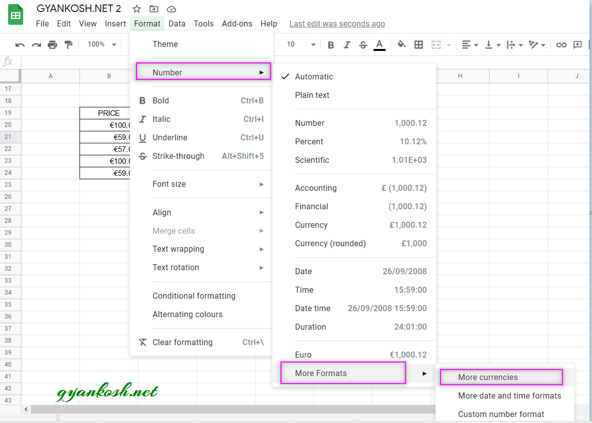
We can reach the same place using the MENU OPTIONS too.
Go to FORMAT > NUMBER >MORE FORMATS> MORE CURRENCIES.
The process is shown in the picture below.
- As we choose MORE CURRENCIES , following dialog box opens up.
- Type the currency symbol name in the SEARCH.
- For our example, we typed EURO and the EURO LISTED UP in the results.
- Click on the result.
- The EURO SYMBOL will appear in front of all the selected cells which contains the numbers.
- The result picture is shown below.

- As we click on the EURO as shown in the previous picture , the EURO SYMBOL will appear in front of all the selected cells which contains the numbers.
- The result picture is shown below.