INTRODUCTION
In practical applications, in maximum cases , we have a large data which can’t be managed by just having a look on the data and manually selecting it.
If we want to search for a particular data, we can do that by using control + F and then typing but it is again a cumbersome task to use it over and again and type the search word.
Or some other ways are to sort the data with respect to some column but in that case too, we’ll need to eliminate the non required data. But after processing the concerned data this time, we again need to bring back the other data. It is again not a very optimum way to manage the data. So , for such situations , to analyze the data by just selecting a particular field and concentrating on concerned data only, we have got this option named FILTER.
Filtering the data is another one of the widely used options in GOOGLE SHEETS . It gives us the facility of instantly opting to see any particular class of data and seeing only what is needed.
BUTTON LOCATION FOR FILTERING DATA IN GOOGLE SHEETS
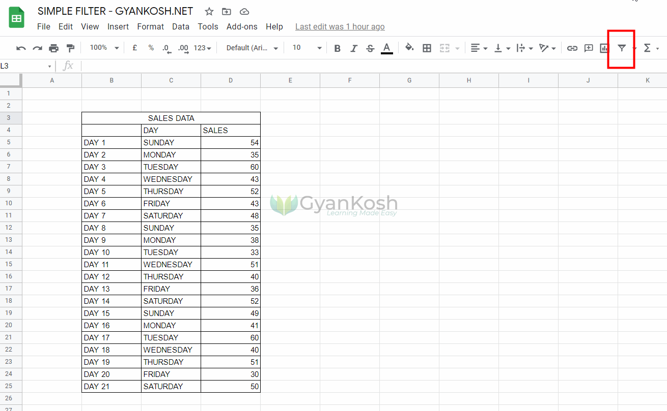
The button location for the FILTER OPTION is shown in the picture below. The filter button is present in the standard toolbar in the right side.
The visual location is shown in the picture below.
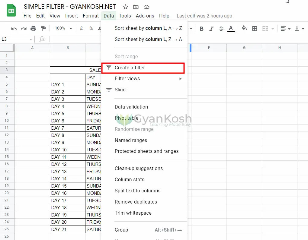
The Filter option is also found under the DATA MENU as shown in the picture below.
STEPS TO APPLY FILTER ON DATA IN GOOGLE SHEETS
The following steps are used to apply a FILTER on any data.
STEPS:
- Select all the COLUMN HEADERS. The complete row can also be selected. It’ll apply filters only on the columns with data but if by chance there is some data in some unintended column, a filter will be given there also. So it is better to select the column headers only.
- Click FILTER BUTTON on the toolbar or go to DATA MENU and choose CREATE A FILTER .
- The filter will be applied on the table.
- Take care that there is no gap between the headers and the data. The filter will be applied on all the contiguous ( Adjacent) data.
- The picture below shows the applied filter. The arrows appear in the right corner of the headers.
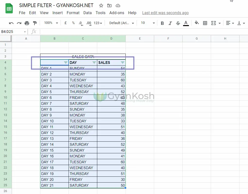
The above picture shows a FILTER APPLIED on the table. The arrows in the lower right corners shows that the filter has been applied.
The data shows the number of vehicles sold on the days of a week.
.
WHEN TO USE FILTER ON DATA
Let us see in which conditions we should use filter on our data.
We can apply different types of operations on the filtered data such as sum,subtraction etc. but the formulas should not be applied on the filtered data. If formulas are applied, it takes into account all the rows hidden in between. But we can check the sum etc. or search any specific information for the filtered data.
READ ME…
Filtering option just hides the rows which do not fulfill the conditions. So never apply any kind of operation. Its just for analyzing the data.
EXAMPLE TO APPLY A FILTER ON DATA
LET’S UNDERSTAND THE DIFFERENT PROCEDURES OF FILTER USING A DATA SAMPLE.
We have a number of vehicles delivered every day of week for three week. Now lets apply different filtering options on the data.
The given data is
| SALES DATA | ||
| DAY | SALES | |
| DAY 1 | SUNDAY | 54 |
| DAY 2 | MONDAY | 35 |
| DAY 3 | TUESDAY | 60 |
| DAY 4 | WEDNESDAY | 43 |
| DAY 5 | THURSDAY | 52 |
| DAY 6 | FRIDAY | 43 |
| DAY 7 | SATURDAY | 48 |
| DAY 8 | SUNDAY | 35 |
| DAY 9 | MONDAY | 38 |
| DAY 10 | TUESDAY | 33 |
| DAY 11 | WEDNESDAY | 51 |
| DAY 12 | THURSDAY | 40 |
| DAY 13 | FRIDAY | 36 |
| DAY 14 | SATURDAY | 52 |
| DAY 15 | SUNDAY | 49 |
| DAY 16 | MONDAY | 41 |
| DAY 17 | TUESDAY | 60 |
| DAY 18 | WEDNESDAY | 40 |
| DAY 19 | THURSDAY | 51 |
| DAY 20 | FRIDAY | 30 |
| DAY 21 | SATURDAY | 50 |
STEPS TO APPLY FILTER
Here are the steps to apply filter on the given data.
- Select all the headers.
- Click FILTER button on the toolbar or go to DATA MENU > CREATE A FILTER.
- Filter will be applied as shown in the picture below.
STEPS TO FILTER THE DATA AS PER THE CRITERIA
Now, after the filter has been applied, let us see how to make the choices from the filters.
We’ll take two examples here for the given data.
- When the sales was greater than 55
- When the sales was greater than 50
vehicles on any day.
STEPS TO FILTER THE DATA AS PER THE CRITERIA
Decide the factor on the basis of which you need to filter the data.
For our example, we want to see the days when the sales was more than 55 and 50 which means SALES column needs to be filtered on the basis of the condition.
- Click the Dropdown symbol on the right side of the SALES COLUMN.
- As we click, a menu with different options will emerge.
- Go to FILTER BY CONDITION.
- Choose GREATER THAN
- Enter 55.
- Click OK at the bottom.
- The output will show only the entries where the sales is greater than 55.
- Again repeat the steps and enter the greater than limit as 50.
- The output will show the entries where the sales is greater than 50.
EXPLANATION:
After applying the filter, the major task remains is to apply the filter on the column which includes the criteria.
we have many ready to use options for the criteria e.g.
Greater Than
Is Empty,
Is Non Empty,
Equal to,
Less than and so on.
Any of these options can be used to filter out the data fulfilling the chosen condition.
The conditions are very easy to understand and ask for the values which can be entered easily with understanding.
HOW TO REMOVE FILTER IN GOOGLE SHEETS?
If we don’t notice any applied filter, it can confuse us many times as the applied rule will be showing only the limited data.
So it is necessary to remove the filter before examining the data.
FOLLOW THE STEPS TO APPLY THE FILTER IN GOOGLE SHEETS
- Simply go to the toolbar and click the FILTER BUTTON, it’ll be ready to remove the filter applied or
- Go to the DATA MENU > TURN OFF FILTER.