Table of Contents
- INTRODUCTION
- WHAT IS WINLOSS SPARKLINE ?
- WHEN SHOULD WE USE WINLOSS SPARKLINE ?
- STEPS TO CREATE WINLOSS SPARKLINES IN GOOGLE SHEETS
- SYNTAX OF SPARKLINE FUNCTION
- EXAMPLE 1: CREATE A WINLOSS SPARKLINE SHOWING THE PERFORMANCE OF EACH TEAM THROUGHOUT THE TOURNAMENT
- SOLUTION:
- EXPLANATION OF THE FORMULA USED:
- ALWAYS REMEMBER
INTRODUCTION
CHARTS are the graphic representation of any data .
Analysis of data is the process of deriving the inferences by finding out the trends, averages etc. about different parameters.
A SPARKLINE is a special type of very compact chart which is created in a single cell.
LEARN THE STANDARD PROCESS OF CREATING SPARKLINE HERE.
These charts are useful in checking the trend with respect to time.
Sparklines are mostly used in a group due to their compactness. Sparklines are just like the charts but very small in size. This is a separate feature from the charts.
Difference between charts and sparklines is that , in a chart, we can create charts using many series but sparkline will create a chart only for one data series.
In this article we’ll learn creating a specific type of sparkline which is known as WINLOSS SPARKLINE only.
WHAT IS WINLOSS SPARKLINE ?
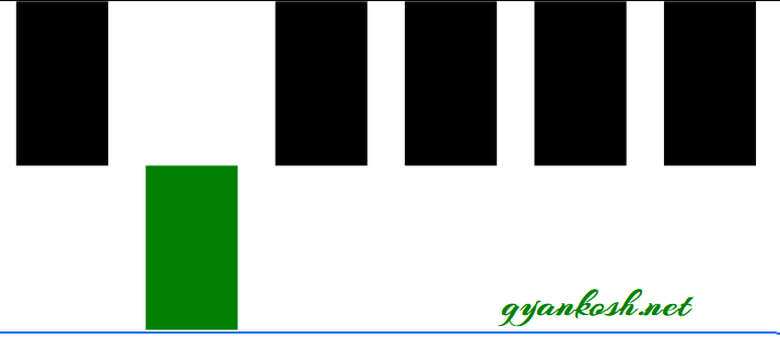
A winloss sparkline is a cell sized chart which only depicts two values, win or loss i.e. a positive value and a negative value.
Have a look at the picture below.
WHEN SHOULD WE USE WINLOSS SPARKLINE ?
WE CAN USE WINLOSS SPARKLINE CHARTS WHEN :
- We need to show only the Two or Three states only i.e. Positive, Absent or Negative.
- When we don’t need to show the levels but the states only.
- Any WIN LOSS situation.
STEPS TO CREATE WINLOSS SPARKLINES IN GOOGLE SHEETS
Kindly first learn the basics here.
LEARN THE STANDARD PROCESS OF CREATING SPARKLINE HERE.
Let us learn to create the sparklines in Google Sheets.
Currently Google Sheets allow the creation of Sparklines using the FUNCTION only and not through any direct access to the graphical interface like the SPARKLINES IN THE EXCEL.
Let us learn the syntax of the WINLOSS SPARKLINE FUNCTION before we use it.
SYNTAX OF SPARKLINE FUNCTION
The syntax of the SPARKLINE FUNCTION is
=SPARKLINE(DATA, {“CHARTTYPE”,”WINLOSS”; OTHER OPTIONS)
- DATA is the range which contains the data for the chart.
- OPTIONS are the different options for customizing our sparkline such as choosing the chart type and other options.
- The options list is given below.
- The options can be put of left blank. If left blank a line chart will be created as the sparkline.
| Winloss sparklines: | |
| PROPERTY | EFFECT |
| color | sets the color of chart columns. |
| lowcolor | sets the color for the lowest value in the chart |
| highcolor | sets the color for the highest value in the chart |
| firstcolor | sets the color of the first column |
| lastcolor | sets the color of the last column |
| negcolor | sets the color of all negative columns |
| empty | sets how to treat empty cells. Possible corresponding values include: zero or ignore |
| nan | sets how to treat cells with non-numeric data. Options are: convert and ignore |
| axis | decides if an axis needs to be drawn (true/false) |
| axiscolor | sets the color of the axis (if applicable) |
| ymin | sets the custom minimum data value that should be used for scaling the height of columns (not applicable for win/loss) |
| ymax | sets the custom maximum data value that should be used for scaling the height of columns (not applicable for win/loss) |
| rtl | determines whether or not the chart is rendered right to left. Options are true or false. |
EXAMPLE 1: CREATE A WINLOSS SPARKLINE SHOWING THE PERFORMANCE OF EACH TEAM THROUGHOUT THE TOURNAMENT
SOLUTION:
The winloss data is shown below.
| MATCH 1 | MATCH 2 | MATCH 3 | MATCH 4 | MATCH 5 | MATCH 6 | |
| TEAM A | 1 | -1 | 1 | 1 | 1 | 1 |
| TEAM B | -1 | 1 | 0 | 1 | -1 | -1 |
| TEAM C | 1 | 1 | -1 | -1 | -1 | 1 |
| TEAM D | 1 | -1 | 1 | -1 | 1 | -1 |
| TEAM E | -1 | -1 | -1 | -1 | -1 | -1 |
Winning is shown by a positive value i.e. 1,
Defeat is shown by a negative value i.e. -1.
A draw is shown by a zero. i.e. 0
IT DOESN’T MATTER IF THE POSITIVE VALUE IS 100 OR 1 , IT’LL CREATE A POSITIVE COLUMN I.E. UPRIGHT COLUMN.
SIMILARLY FOR NEGATIVE VALUES , -1 OR -100, IT’LL CREATE A NEGATIVE COLUMN I.E. INVERTED COLUMN
Now, let us draw the sparklines for all the tems to check out their performance.
STEPS TO CREATE WINLOSS SPARKLINE IN GOOGLE SHEETS
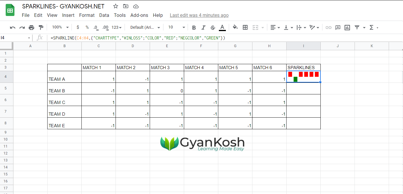
- Select the cell where you want to create the sparkline. For our example, we’ll select the cell I4.
- Enter the formula in the format = SPARKLINE( DATA RANGE, OPTION RANGE OR OPTIONS IN THE SHOWN FORMAT ABOVE”)
- For our example, the formula will be =SPARKLINE(C4:H4,{“CHARTTYPE”,”WINLOSS”;”COLOR”,”RED”;”NEGCOLOR”,”GREEN”})
- Press ENTER and we can see the sparkline for the TEAM A as shown in the picture below.
- Now we have created the SPARKLINE for the first Team.
- For the rest, we can simply drag down the formula and we’ll be all good.
- Click the small square on the right of the selection rectangle , keep the mouse button pressed and drag down through TEAM E.
- All the sparklines will be created for all the teams.
The animation shows the process.
EXPLANATION OF THE FORMULA USED:
Let us discuss the formula used to create our sparkline.
The formula used is
=SPARKLINE(C4:H4,{“CHARTTYPE”,”WINLOSS”;”COLOR”,”RED”;”NEGCOLOR”,”GREEN”})
- The first argument is C4:H4 which is the range of the data.
- The second arument contains the arguments to set the properties of the sparkline.
- CHART TYPE fixes the type to the WINLOSS type of sparkline.
- ; delimits each property from the other.
- COLOR fixes the color of the bars, which we have set to RED.
- NEGCOLOR fixes the color of the negative bars which we have set to GREEN.
You can add as many properties by referring to the table mentioned above.
ALWAYS REMEMBER
WINLOSS type of sparkline takes three types of values.
- POSITIVE
- NEGATIVE
- BLANK
POSITIVE VALUES , WHATEVER BE THE MAGNITUDE OR VALUE, IF IT IS POSITIVE A POSITIVE COLUMN WILL BE SHOWN.
NEGATIVE VALUE, WHATEVER BE ITS MAGNITUDE OR VALUE, IF IT IS NEGATIVE A NEGATIVE COLUMN WILL BE SHOWN.
BLANK WILL KEEP A BLANK SPACE WITHOUT ANY COLUMN. THIS SETTING CAN BE SUPPRESSED TOO.