Table of Contents
- INTRODUCTION
- WHY TO FORMAT THE PHONE NUMBERS IN GOOGLE SHEETS?
- EXAMPLE: HOW TO FORMAT THE GIVEN NUMBER INTO AMERICAN STYLE PHONE NUMBER FORMAT
- EXAMPLE 2: FORMAT THE PHONE NUMBER AS INTERNATIONAL PHONE FORMAT
- HOW TO REMOVE THE PHONE FORMATTING IN GOOGLE SHEETS?
- REMOVE THE PHONE FORMATTING FROM THE GIVEN NUMBERS
- CONVERT PHONE NUMBER FORMATTING INTO NORMAL NUMBERS
INTRODUCTION
Google Sheets can be used for any number of useful applications which are customized as per our requirements.
One such requirement is the PHONE NUMBER KEEPING.
We can create a database of the phone numbers and keep it stored for the readily usage. But what if we want to present the phone numbers in the exact standard phone numbers format.
Well! we can easily do that with the formatting option in Google Sheets.
In this article we’ll learn the way to Format the Phone Numbers in Google Sheets.
WHY TO FORMAT THE PHONE NUMBERS IN GOOGLE SHEETS?
With time, every frequently used information has been given a standard format which gives the information a certain recognition.
For example, if a number is written as 555.00 , we’ll take it as a currency, 5’11”, we’ll take it as height and so on.
Similarly, (800) 555-0199 will represent a telephone number.
What if we format the field in such a way that we need not take care about the format?
Let us learn the way to format the telephone number automatically in the prescribed format.
EXAMPLE: HOW TO FORMAT THE GIVEN NUMBER INTO AMERICAN STYLE PHONE NUMBER FORMAT
The format shown above (800) 555-0199 is the phone number format prominently used in US mainly.
In addition to this, we have many other formats only such as local, domestic, international and more which we’ll be discussing below.
Let us learn the way to format the given numbers in the american phone format.
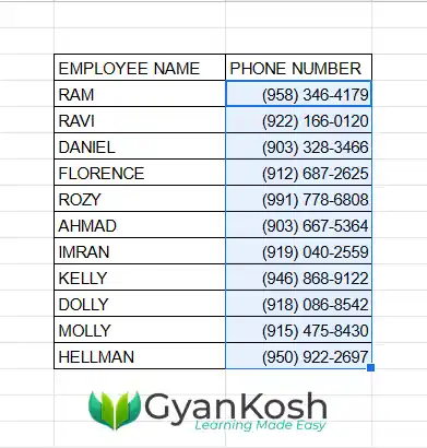
Have a look at the data given below.
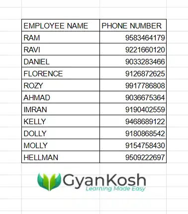
The given data simply contains the names of the employees and their phone number.
Let us try to format them as per our requirement.
STEPS TO FORMAT THE NUMBERS INTO PHONE NUMBERS
- Select the cells containing the phone numbers.
- Go to FORMAT MENU and choose NUMBERS> CUSTOM NUMBER FORMAT as shown in the picture below.
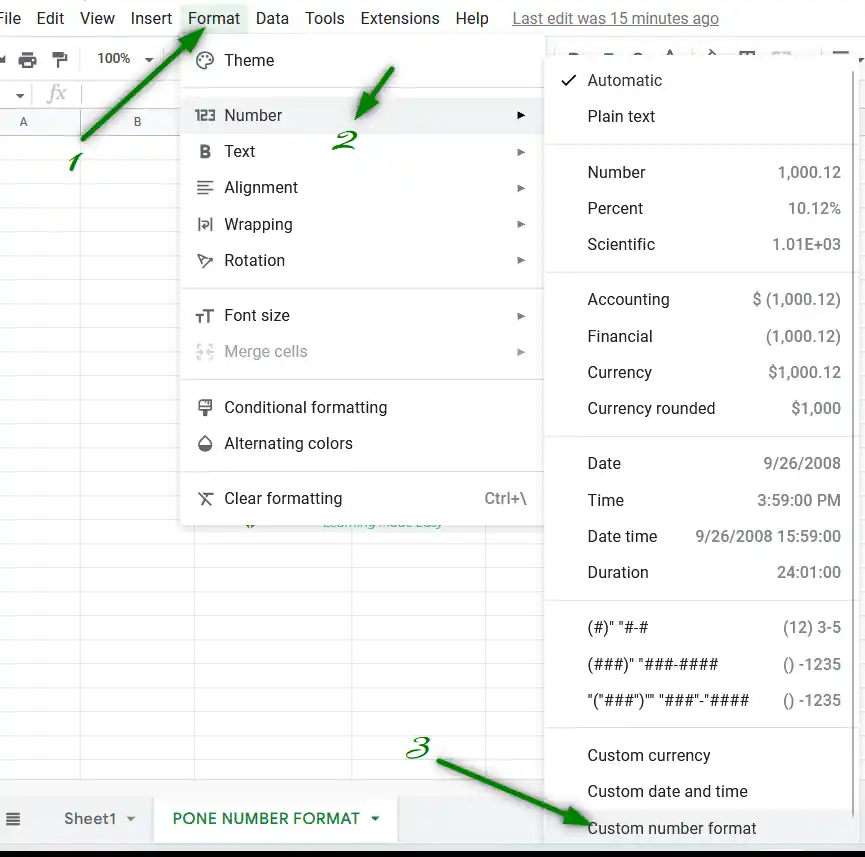
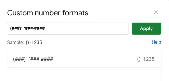
- As we click CUSTOM NUMBER FORMAT, a new window will open.
- Enter the format as (###)” “###-####.
- Click APPLY.
- As we click Apply, the format will be applied to the selected cells.
- The result is shown below.
EXAMPLE 2: FORMAT THE PHONE NUMBER AS INTERNATIONAL PHONE FORMAT
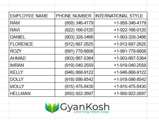
The international phone number format can be shown as +1-212-486-7899 where the first number with a + sign represent the country code.
Let us format the given phone numbers as per the international format.
In this process, most of the steps are same and only the last step i.e. using the Custom format is different.
FOLLOW THE STEPS TO FORMAT THE INTERNATIONAL PHONE NUMBERS
- Follow the steps of EXAMPLE 1 from Step 1 to Step 3.
- Enter the custom format as +#-###-###-####
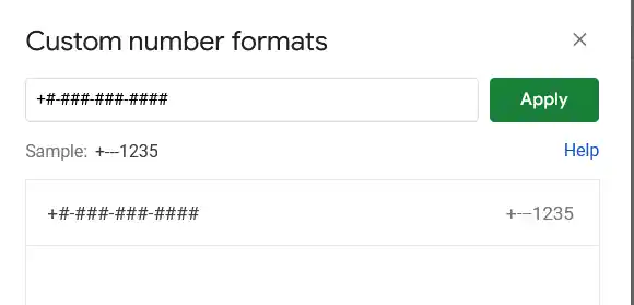
- This format will place the digits at every #.
- It’ll also adjust the country code for two digits in the same format and won’t create any issue.
HOW TO REMOVE THE PHONE FORMATTING IN GOOGLE SHEETS?
What if we want to remove the phone number formatting from the given numbers.
We may have two cases .
- The given numbers are in the phone formatting only.
- The numbers are in the phone formatting as text.
Both of these cases are different as in the phone formatting, it is only the custom formatting and not the text, whereas the number which is in phoneformat but stored as text needs to be taken care in a separate way.
We’ll discuss both.
REMOVE THE PHONE FORMATTING FROM THE GIVEN NUMBERS
If the phone numbers are simply custom formatted as we did in the article above, follow the steps to remove the phone formatting in Google Sheets.
- Simply select all the cells from where you want to remove the phone formatting.
- Go to FORMAT MENU> NUMBER > AUTOMATIC as shown in the picture below.
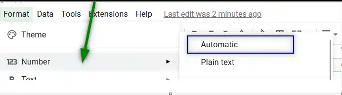
- As we choose this option, the custom phone number formatting will be removed from all the numbers and they’ll appear to be the normal numbers.
CONVERT PHONE NUMBER FORMATTING INTO NORMAL NUMBERS
Now, if your numbers are not custom formatted but written as text , we need to apply a different method to remove the formatting.
FOLLOW THE GIVEN STEPS TO CONVERT THE PHONE NUMBERS WRITTEN AS TEXT INTO NUMBERS
- Select all the cells containing the phone numbers.
- For this way, we need to use a second column which we may call as a helper column.
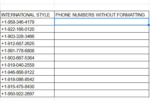
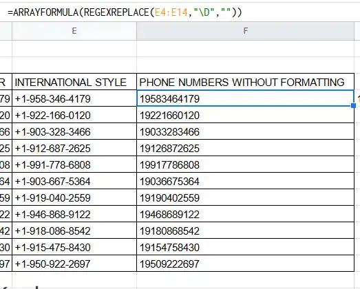
- In the helper column, enter the formula as =ARRAYFORMULA(REGEXREPLACE(E4:E14,”\D”,””)) where E4:E14 is the range which contains the phone numbers containing cells.
- Press Enter.
- The result will appear which will contain only numbers without any other character.
- The result is shown below.