INTRODUCTION
GOOGLE SHEETS allows us to use many DIRECT-TO-USE functions which we can use to get the desired output. Even after having a large number of functions, certain situations may arise when we don’t find the apt function to be used.
For such situations, we need to use more than one function in conjunction which will allow us to find out the solution to those problems.
One of such issue is counting the duplicate values.
In this article, we’ll try to find out the solution to count the duplicate items in Google Sheets.
WHAT ARE DUPLICATE ITEMS?
DUPLICATE ITEMS are the ones which are repeated in the given data.
Duplicate items are the ones which have exactly two copies in the given data.
For example, in the following data
1 2 3 2 4 5 6 7 8 9 12 13 14 15 16 17 18
2 is the value which is a duplicate item.
After that we have understood, let us find out the way to count the values which have their duplicates in the given data.
EXAMPLE 1: COUNT DUPLICATE VALUES IN GOOGLE SHEETS
Let us take an example to demonstrate the same.
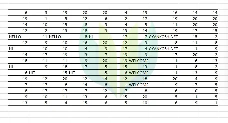
The following data contains some random numbers and text values.
We need to find out the number of values which occur twice i.e. duplicates.

FOLLOW THE STEPS TO FIND OUT THE DUPLICATE VALUES IN GOOGLE SHEETS:
- Double click the cell where you want the result.
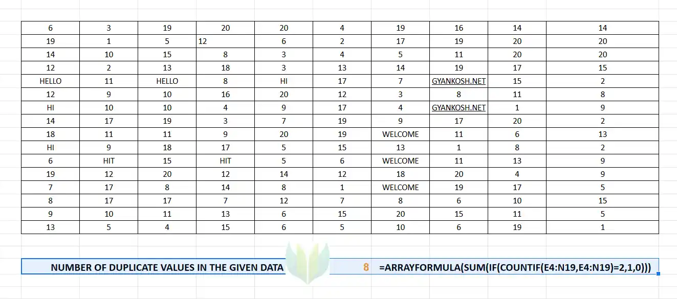
- Enter the function as =ARRAYFORMULA(SUM(IF(COUNTIF(E4:N19,E4:N19)=2,1,0))).
- Press ENTER.
- The result will appear as 8. i.e. 8 duplicate values are present in the given data. [4 PAIR]
The following picture shows the result.

EXPLANATION:
The formula used in the above problem is =ARRAYFORMULA(SUM(IF(COUNTIF(E4:N19,E4:N19)=2,1,0))).
The COUNTIF FUNCTION works for the complete range i.e. E4:N19 and searches for the complete range and result in the frequency of the particular value. As this is an arrayformula, it’ll search all the values.
We compare the frequency or count of a particular value and compare it with 2, i.e. the values which are duplicates and replace it with 1 using the IF FUNCTION.
Finally , after the complete processing the values are passed to the SUM FUNCTION which totals the values and provides the result.
CHECKING THE RESULTS:
We can check the result using the CONDITIONAL FORMATTING.
Use the custom rule and enter the formula as =COUNTIF($E$4:$N$19,E4)=2.
It’ll highlight all the values which are duplicate.
We can check that 8 values are duplicates. [ 4 pairs].
The following picture shows the highlighted values.
