Table of Contents
INTRODUCTION
After we created a pivot table in Excel, which is a powerful and fast deployment of tabular data which provides us with many ready-to-use functionalities.
Sorting is one of the frequently used features in spreadsheet applications.
As we know, SORTING IS ARRANGING DATA IN A PARTICULAR FASHION WHICH CAN BE ASCENDING OR DESCENDING or A to Z or Z to A.
Sorting is very beneficial in many of the required operations in a spreadsheet application.
Let us learn the way to use this option in the pivot tables.
EXAMPLE: PIVOT TABLE
Let us create a pivot table with a few fields on which we can try our sorting.
For example, let us take an example of the Sales and other data over a few months.
We’ll be creating a pivot table of the given data and sort a few fields in the resulting pivot table.
| MONTH | SALES | ENQUIRIES |
| JANUARY | 56 | 118 |
| FEBRUARY | 60 | 163 |
| MARCH | 55 | 164 |
| APRIL | 73 | 150 |
| MAY | 63 | 161 |
| JUNE | 51 | 168 |
| JULY | 75 | 154 |
| AUGUST | 67 | 109 |
| SEPTEMBER | 71 | 113 |
| OCTOBER | 73 | 125 |
| NOVEMBER | 61 | 198 |
| DECEMBER | 51 | 108 |
CREATING A PIVOT TABLE IN EXCEL
- Select the given data and go to INSERT TAB and Click PIVOT TABLE.
- Choose CREATE PIVOT TABLE on a new sheet.
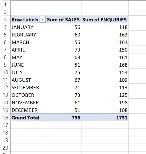
- Click on the PIVOT TABLE and choose all the fields so that our pivot table look like as the one shown below.

HOW TO SORT PIVOT TABLE IN EXCEL
Let us sort the given pivot table with respect to the column sum of ENQUIRIES.
We can sort pivot tables using
- RIGHT CLICK METHOD
- RIBBON OPTION METHOD
1.RIGHT CLICK METHOD TO SORT PIVOT TABLE IN EXCEL
FOLLOW THE STEPS TO SORT THE PIVOT TABLE
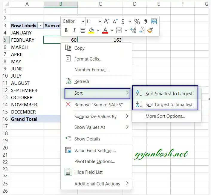
- Simply right-click the column you want to sort.
- Choose SORT> SORT SMALLEST TO LARGEST or LARGEST TO SMALLEST.
- The pivot table will get sorted.

- Simply use the option and the data will be sorted.
You need not select the data as we need in the normal procedure. Sorting will be applied to the complete pivot table.
2. USING RIBBON OPTION TO SORT PIVOT TABLE IN EXCEL
We can sort pivot data using the SORT OPTION available in the ribbon also.
FOLLOW THE STEPS TO SORT PIVOT TABLE IN EXCEL USING RIBBON OPTION:
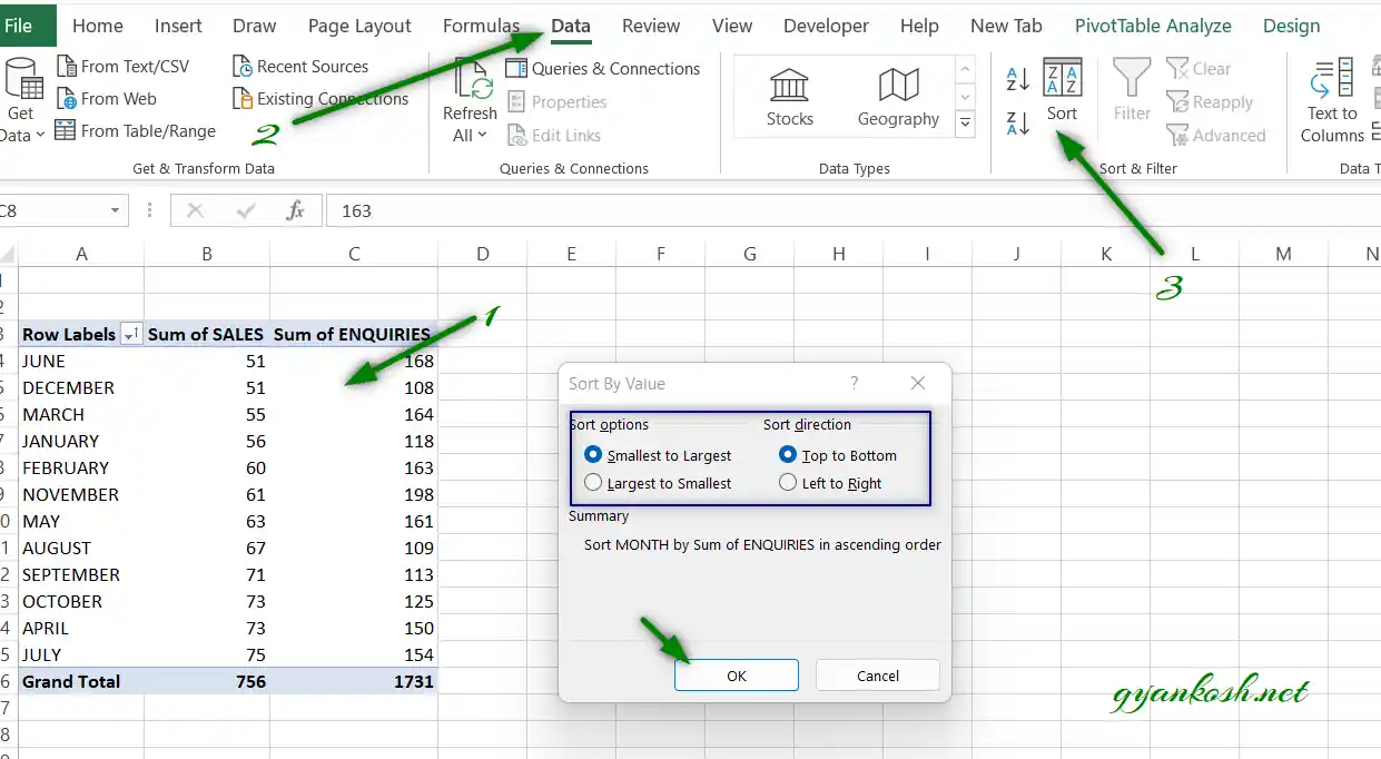
- Click on the the column which will be the basis of sorting.
- Go to DATA TAB and click on SORT.
- A new small window for further options will open as shown in the picture below.
- Make the settings as per requirement and click OK.

- As we click OK, the PIVOT TABLE will be sorted.