Table of Contents
- INTRODUCTION
- WHEN TO HIGHLIGHT THE DUPLICATES IN MICROSOFT EXCEL?
- STEPS TO HIGHLIGHT THE DUPLICATES IN EXCEL
- STEPS TO HIGHLIGHT DUPLICATES IN EXCEL
- EXPLANATION OF THE METHOD TO HIGHLIGHT THE DUPLICATE CELLS IN EXCEL
INTRODUCTION
While analyzing the data, we might come across the repeated data which needs to be replaced or highlighted. If we start doing this process manually, it can be done on a small range or data but what if we have thousands of rows to be examined. Obviously, it is going to be almost impossible. That is the reason why we need to find and replace the duplicate entries.
We can easily remove the duplicate entries using the available tools in EXCEL.
But, there is always a doubt we simply remove the duplicates.
What if we just want to highlight the duplicates in a specified column and check them manually.
There is no direct utility for such operation. So, in this article we would try to find out a way to ONLY HIGHLIGHT the repeated values in a specified column using CONDITIONAL FORMATTING.
Let us start.
WHEN TO HIGHLIGHT THE DUPLICATES IN MICROSOFT EXCEL?
HIGHLIGHTING THE DUPLICATES in a specified column can be very useful while analyzing any data.
For example,If there are few cases in which the principal field is same but other data is different or we want to check the duplicate values in any column which we want to remove and many other requirements.
In such cases we can use the process to highlight the duplicates.
STEPS TO HIGHLIGHT THE DUPLICATES IN EXCEL
Let us take an example of a column containing few duplicate entries.
Suppose the following data is present in the column.
APPLE
BANANA
POMEGRANATE
OLIVE
BANANA
APPLE
GRAPES
GUAVA
WALNUT
CASHEW
ALMONDS
Our aim is to just highlight the entries which are repeated. [Only highlighting the entries which are repeated so that we don’t need to focus upon the entries which are already unique. ]
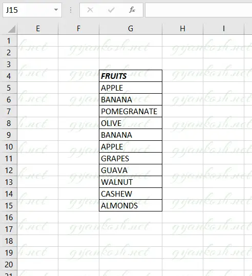
It is clearly visible that few of the entries shown in the above data is duplicate for example, apple, banana etc.We will first use the conditional formatting to highlight the data followed by the explanation of the formula.
STEPS TO HIGHLIGHT DUPLICATES IN EXCEL
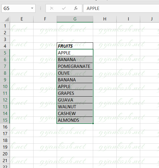
STEP 1:
- Select the column or all the cells in which we want to highlight the duplicate items.
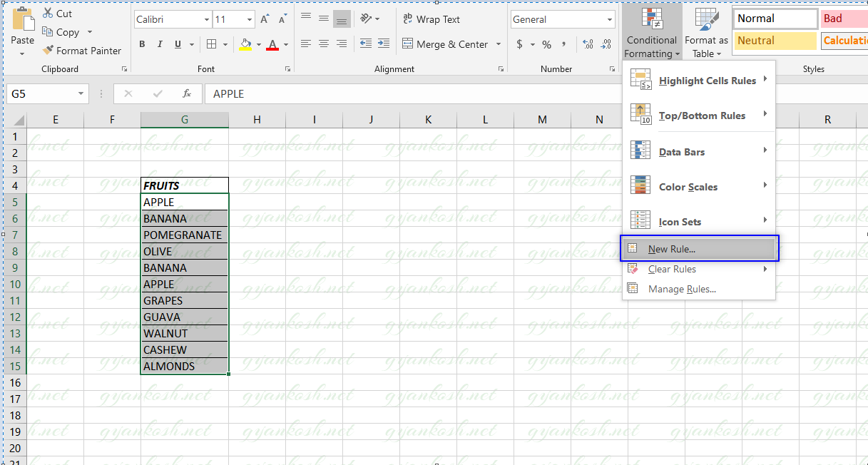
STEP 2:
- Go to HOME TAB > Conditional Formatting .
- Choose NEW RULE from the CONDITIONAL FORMATTING drop down list.
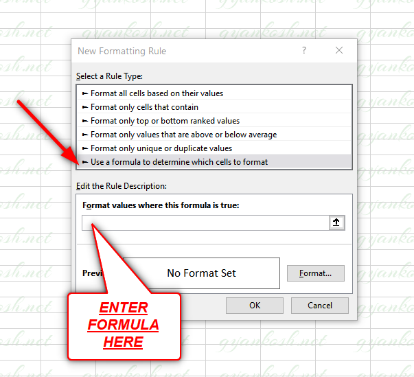
The following picture shows the NEW FORMATTING RULE DIALOG box which will appear after choosing the NEW RULE option from the drop down.
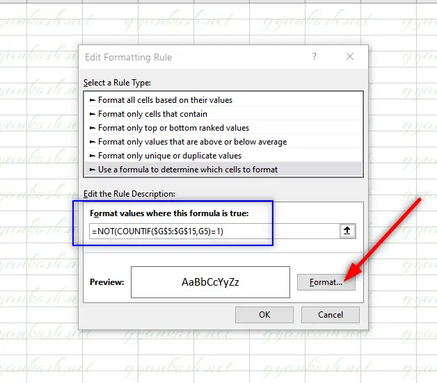
In the dialog box choose USE A FORMULA TO DETERMINE WHICH CELLS TO FORMAT, the last option which is shown by a RED ARROW in the following picture.
STEP 3:
- ENTER THE FORMULA AS =NOT(COUNTIF($G$5:$G$15,G5)=1) [EXPLANATION IN NEXT SECTION]
- After we have entered the formula, we have to select the format for the HIGHLIGHTED CELLS.
- Click FORMAT BUTTON as marked by the RED ARROW in the following picture.
STEP 4:
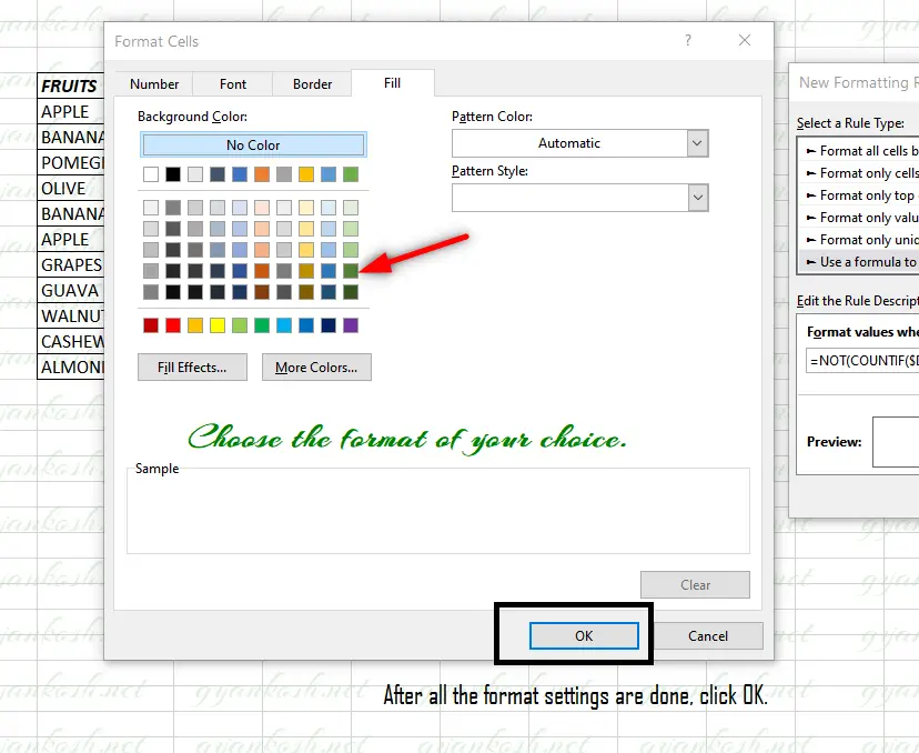
- After clicking the FORMAT BUTTON, the FORMAT CELLS dialog box will open.
- Select the format [ FILL COLOR, FILL EFFECT, PATTERN, PATTERN STYLE, FONT,BORDER ETC. ] which you want to be the format of the highlighted cells.
- For our example, we have just chosen the FILL COLOR as OLIVE GREEN.
- After choosing the format, click OK.
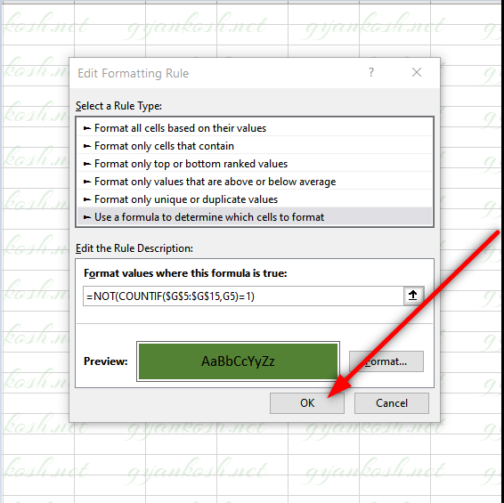
STEP 5:
- After clicking OK, we’ll again reach back to EDIT FORMATTING RULE dialog box with the final settings as shown in the picture below.
- Click OK.
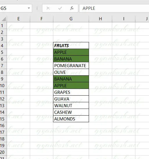
STEP 6:
- After clicking OK, the final result will appear.
- All the repeated values will be highlighted.
EXPLANATION OF THE METHOD TO HIGHLIGHT THE DUPLICATE CELLS IN EXCEL
CONDITIONAL FORMATTING is a very useful option present in EXCEL.
Conditional formatting provides us with the option of HIGHLIGHTING the specific cells within our data which fulfills the certain given conditions.
In our example, we want to highlight the duplicate data for which we used a CUSTOM FORMULA.
The formula used is
=NOT(COUNTIF($G$G5:$G$15,G5)=1)
Let us understand the formula.
The internal function is simple COUNTIF FUNCTION which counts the cells containing a particular data with the given condition.
In this we put the range as the complete data with the absolute references using the $. [ Absolute references are the ones which doesn’t change while dragging down the formula or any relative action as in conditional formatting.]
The value to be looked up is given as D6 which is the first cell in our selection.
IN CONDITIONAL FORMATTING, THE FORMULA IS ALWAYS PUT FOR THE FIRST CELL OF THE SELECTED RANGE.
The outcome of countif is equated to 1 which means that we are asking the EXCEL to tell us whether the number of occurrences of data is equal to 1 or not.
If yes, then we don’t want a highlight and if no, then we want a highlight.
So we used the NOT function which simply reverses the outcome from true to false and false to true which solves our problem.