INTRODUCTION
RIBBON is the name given to the new layout of controls which was introduced in MICROSOFT OFFICE 2007. Since then it has become a signature look and feel of MS OFFICE TOOLS.
If you have used any version of MS TOOLS after 2007, you must have looked at it and used a number of features present there.
RIBBON IS THE AREA AT THE TOP OF THE MS OFFICE TOOLS SUCH AS EXCEL, WORD, POWERPOINT ETC. WHICH CONTAINS ALL THE CONTROL BUTTONS CLASSIFIED INTO TABS AND GROUPS.
The design was a major change in the regular MENU TYPE window designs which are considered kind of boring today.
Let us find out some interesting features about the ribbon such as customizing the ribbon, hiding or showing extra features in the ribbon, creating own tab in the ribbon and much more.
WHAT IS A RIBBON IN MICROSOFT EXCEL
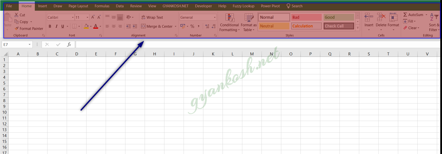
RIBBON is a dedicated area laid down on the top of the working window [sheet] just like the toolbars in the MS OFFICE TOOLS or Microsoft Excel. The space contains many useful functions under many TABS [ just like menus] and grouped under sub sections.Look at the picture below.
WHERE IS RIBBON LOCATED IN MICROSOFT EXCEL
RIBBON is located on the top of the working area [ cells or sheet ]. The reference picture is shown in the previous section.

HOW TO HIDE THE RIBBON IN MICROSOFT EXCEL
The Ribbon can be hidden or shown as per the choice if required.The need for showing or hiding ribbon can arise if we need more visible space in the worksheet.
Follow the steps to HIDE THE RIBBON.
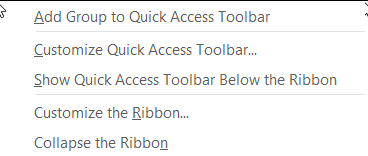
- RIGHT CLICK anywhere on the Ribbon.
- The following right click menu will open.

- Choose COLLAPSE THE RIBBON.
- It’ll hide the ribbon and the workspace will increase.

HOW TO SHOW THE RIBBON IN MICROSOFT EXCEL
We can easily SHOW the ribbon if it is hidden in the same way we hid the ribbon in the previous section.The need for showing or hiding ribbon can arise if we need more visible space in the worksheet.
Follow the steps to SHOW THE RIBBON.
- RIGHT CLICK anywhere on the Ribbon.
- The following right click menu will open.
- Choose COLLAPSE THE RIBBON and uncheck it by clicking on it.
- It’ll unhide the ribbon and it will be restored.
HOW TO SHOW OR HIDE ANY TAB IN RIBBON OF MICROSOFT EXCEL
The ribbon has a standard format when we have a newly installed MICROSOFT EXCEL in our system. But we can customize the ribbon easily.
We can add , customize or remove any command or tab from the ribbon as per our choice.
Let us learn to Show or Hide any Tab from the ribbon.
Follow the steps to SHOW OR HIDE a tab from the ribbon in Microsoft Excel.
If we want to add the commands, follow the steps.
- Right Click on the ribbon and choose CUSTOMIZE THE RIBBON or go to FILE>OPTIONS>CUSTOMIZE RIBBON [Shown in the picture below ].
- Both options will take us to the same location.
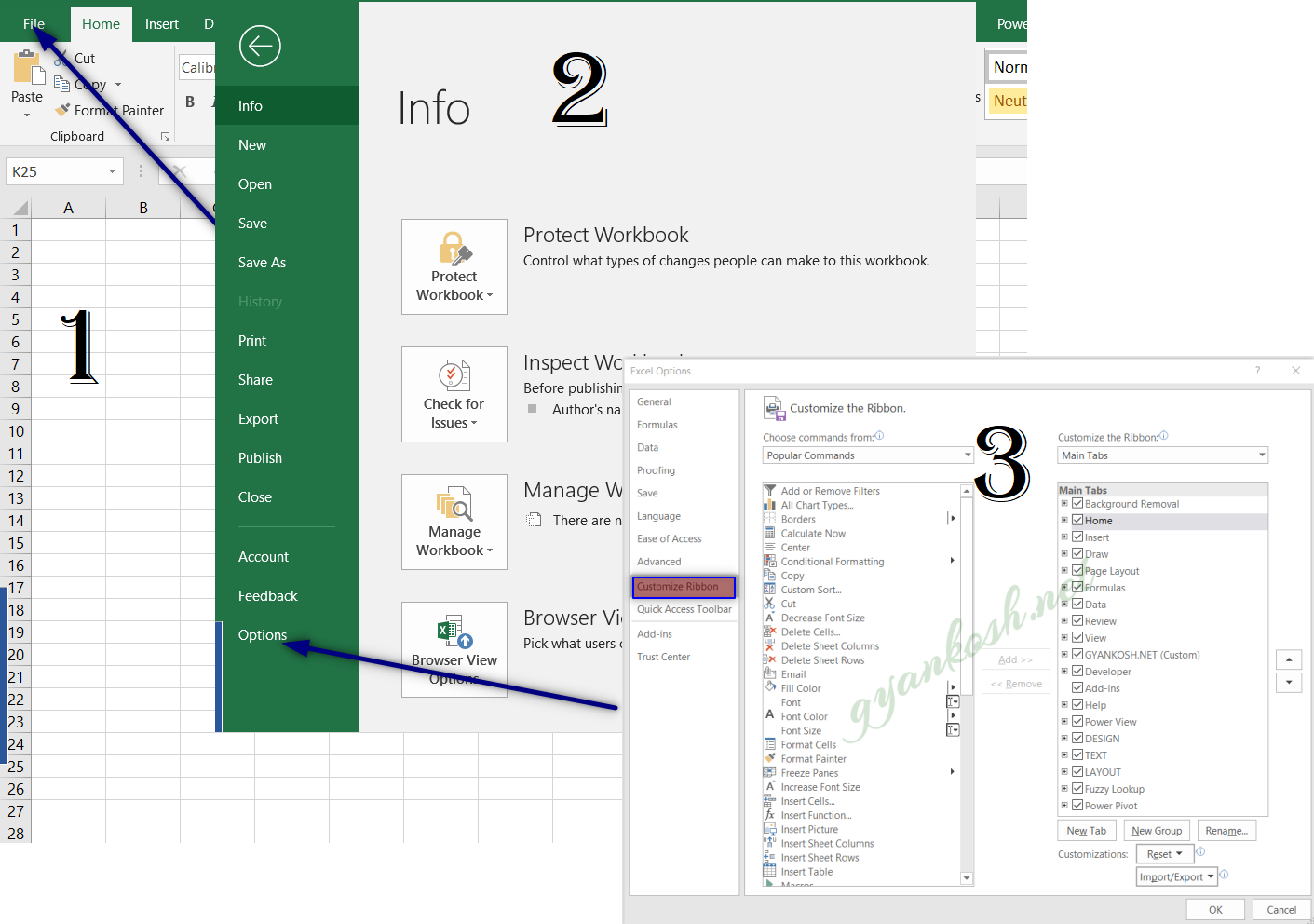
After choosing the option CUSTOMIZE THE RIBBON either by RIGHT CLICKING the RIBBON or through the FILE MENU, following option opens up.
Have a look at the picture below.
EXCEL OPTIONS has the selection for the CUSTOMIZE RIBBON which is a completely separate option available.
The option consists of two lists.
The left list contains all the commands available and the right list contains the Present Layout and the selected options for the Ribbon.
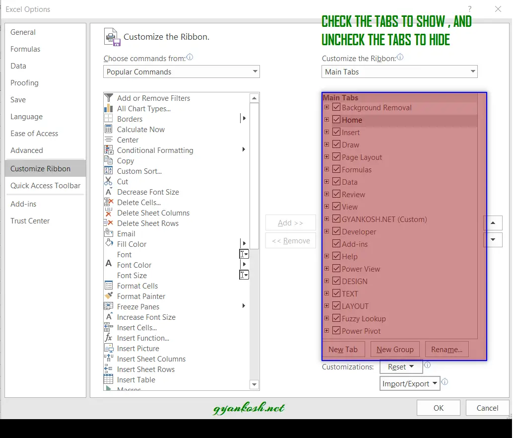
SHOW ANY TAB ON THE RIBBON:
- Select the option from the Right Side List.
- The selected option will be visible in the Ribbon.
HIDE ANY TAB ON THE RIBBON:
- Deselect any option from the Right Side List.
- The deselected option will be removed from the Ribbon.
HOW TO ADD ANY NEW OR CUSTOM COMMAND IN THE RIBBON
If we have a created a new functionality like a Macro or Function etc. , it would be great if we could find these options in the Tab itself.
EXCEL gives us the option of creating our own TAB and putting any additional commands or the custom commands in the Tab.
If we want to change the order of the commands, follow the steps.
- Reach the CUSTOMIZE RIBBON option using any of the method discussed in the previous sections. [Right Click or through File menu ]
- Select the Tab in the MAIN TABS list [RIGHT SIDE LIST ] , after which you want to insert the new tab.
- Click NEW TAB in the lower right portion of the EXCEL OPTIONS [customize ribbon option ].
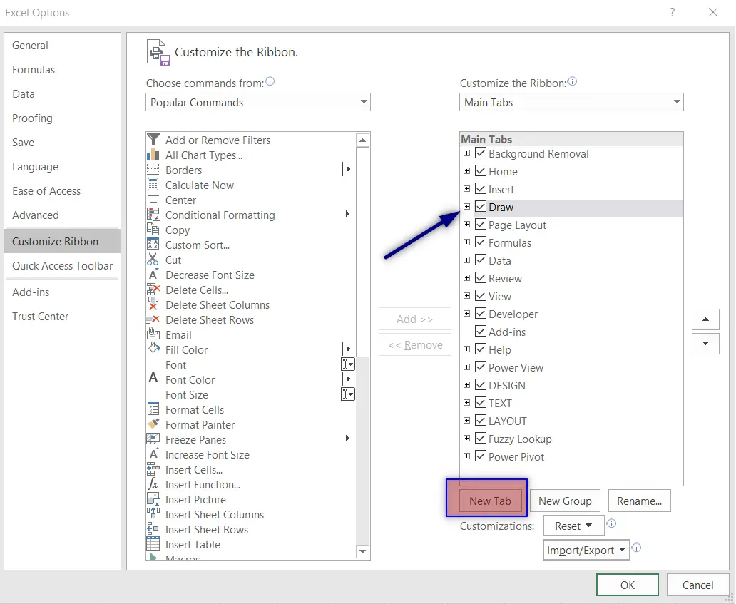
- As we click NEW TAB, a NEW TAB is created just after the Tab we have selected.
In the picture above, we have selected the DRAW TAB, so the new tab is inserted just below the DRAW TAB. Refer to picture below.
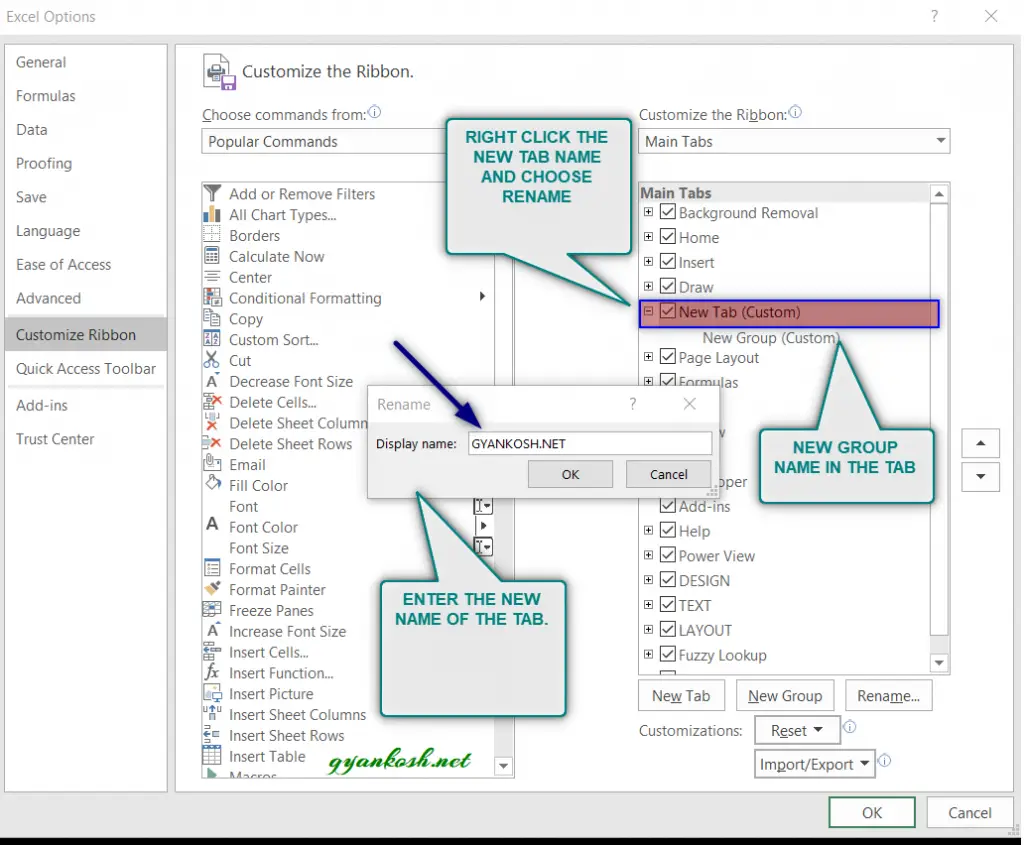
After the NEW TAB has appeared in the MAIN TABS , its time now to change the name of the Tab as per your choice.
CHANGING THE NAME OF THE NEW TAB IN RIBBON:
- RIGHT Click on the NEW TAB(Custom).
- Choose RENAME option.
- Excel will ask for the New Display Name.
- Enter any desired name. For our example we have entered GYANKOSH.NET [REFER PICTURE BELOW]
- Click OK.
- The New Tab name has been renamed as GYANKOSH.NET
After Renaming the NEW CUSTOM TAB, the situation is something like this.
We have a new empty TAB named GYANKOSH.NET.
Now, let us change the GROUP NAME also.
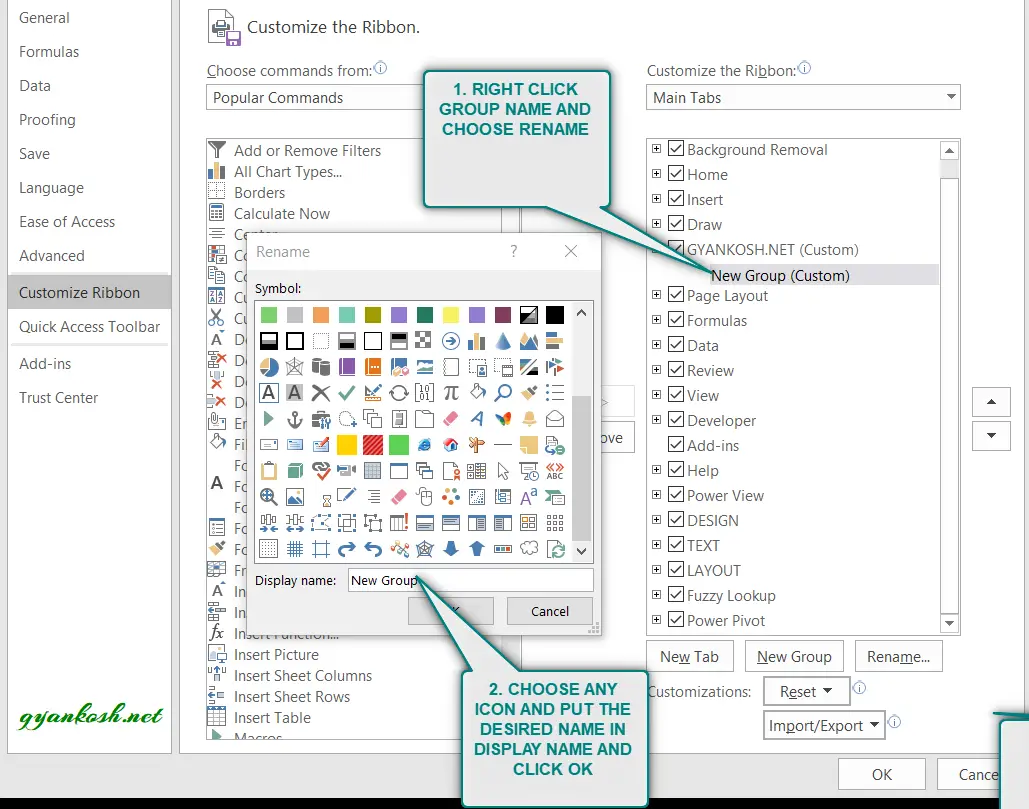
CHANGING THE NAME OF THE GROUP IN RIBBON:
- Right Click the GROUP NAME and choose RENAME.
- RENAME option will open a dialog box asking for the SYMBOL CHOOSE and GROUP NAME.
- Choose the symbol as you like and put the GROUP NAME as required.
- Click OK.
- For our example, we have given the group name as “gyankosh.net”.
- [ BUT THE NAME OF THE GROUP WON’T BE VISIBLE YET AS WE HAVE NOT ADDED ANY FUNCTIONALITY TO OUR NEWLY CREATED TAB]
- REFER THE PICTURE BELOW FOR REFERENCE.
Till now we have already created a new CUSTOM TAB in RIBBON of MICROSOFT EXCEL and a group named gyankosh.net.
Now, let us add some functions to this tab so that we can save our time by directly using these functions.
REFER TO THE PICTURE GIVEN BELOW.
On the left hand side, there is a long list of AVAILABLE OPTIONS which can be put in our custom tab.
At the top there is a drop down [ mentioned in the picture too ] from which we can select the group of the commands available as per choice. For example
POPULAR COMMANDS,
ALL COMMANDS,
COMMANDS NOT IN THE RIBBON , MACROS, ETC.
If you want to select from the complete exhaustive list of the options, go for ALL COMMANDS.
CHOOSING THE COMMANDS AND ADDING THEM TO THE TAB.
- Select the group on the Right side List. [ The group in which we want to enter the particular command. There can be multiple groups which can be created under a tab by clicking right and choosing ADD NEW GROUP.]
- After selecting the TARGET GROUP on the right side, we are ready to choose and add the commands to our newly created group under our custom tab.
- Select ALL COMMANDS from the DROP DOWN at the top.
- Now, choose the command , select it and click ADD, which will shift the command from the left hand side [ which is just like a pool of available commands ] to our new group. [gyankosh.net named group ].
- Repeat the process till you have put all the commands you want in your new tab.
- Click OK.
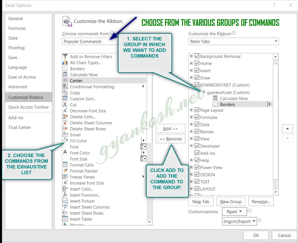
After you have selected and Added all the commands you want, Click OK at the bottom and we are done.
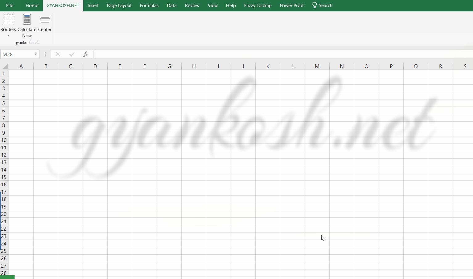
For our example, we have taken three commands namely CALCULATE NOW, BORDERS, CENTER.
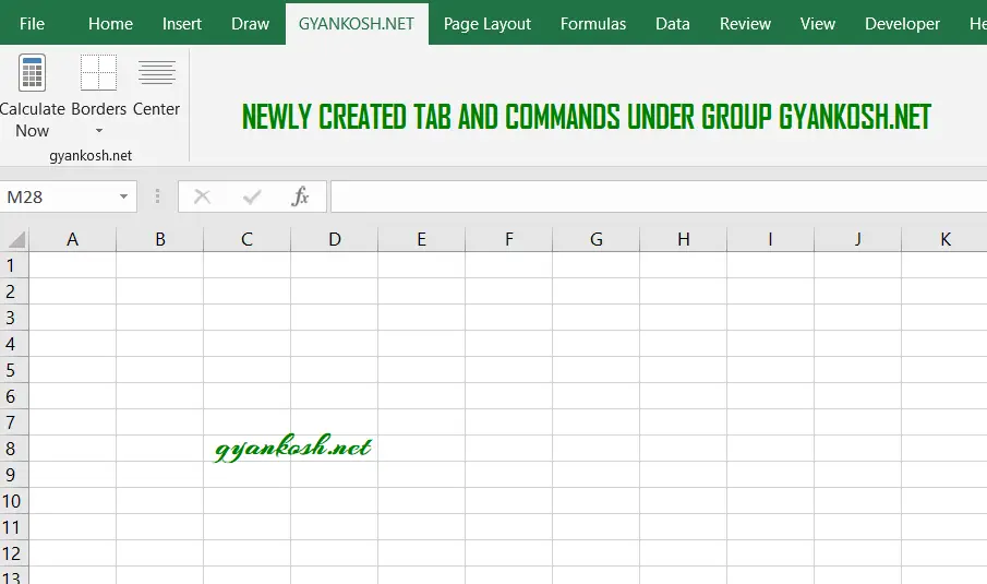
The following picture shows the NEW CUSTOM TAB which contains the commands as per our choice.
HOW TO RESET RIBBON LAYOUT IN MICROSOFT EXCEL
Suppose , we have created a lot of changes and we want to RESET all the customization of the RIBBON. [ Resetting is the process of bringing the custom things back to the original state].
If we want to reset the RIBBON CUSTOMIZATION , follow the steps.
RIGHT CLICK the RIBBON and choose CUSTOMIZE THE RIBBON option or reach through the FILE MENU> EXCEL OPTIONS > CUSTOMIZE RIBBON.
- At the RIGHT BOTTOM, we can see the option of RESETTING.
- Choose the RESET ALL CUSTOMIZATION from the RESET DROP DOWN and click OK.
- The RIBBON will be reset to its original state. [Including the DEVELOPER TAB ].
- The animation below depicts the process.