Table of Contents
- INTRODUCTION
- WHAT IS DATA VALIDATION IN EXCEL?
- WHEN DO WE USE DATA VALIDATION IN EXCEL?
- WHERE IS DATA VALIDATION OPTION OR BUTTON IN EXCEL 2013,2016,2019,2021 ?
- EXAMPLE: USE DATA VALIDATION IN EXCEL
- PUTTING THE CONDITION IN PLACE:
- ENTERING THE INPUT MESSAGE:
- ENTERING THE ERROR ALERT MESSAGE:
- RUNNING THE EXAMPLE
- VALIDATE ALREADY FILLED DATA USING DATA VALIDATION
- EXAMPLE:
- STEPS TO HIGHLIGHT INVALID DATA
- REMOVING DATA VALIDATION IN EXCEL
- FAQs
- HOW TO APPLY DATA VALIDATION TO WHOLE COLUMN?
- HOW TO REMOVE DATA VALIDATION FROM A COLUMN?
- HOW TO APPLY DATA VALIDATION ON MULTIPLE COLUMNS?
- HOW TO APPLY DATA VALIDATION ON MULTIPLE CELLS?
INTRODUCTION
Excel is a great tool that provides countless useful tools for data analysis. In addition to this, it has great tools for making wonderful reports, charts, etc. Out of these features, one of the features is DATA VALIDATION which helps us control the data entered in the cell and provide useful information for our users.
Data validation means checking the data before entering. It gives us the power to condition the values which can be entered and rejected into any cell.
WHAT IS DATA VALIDATION IN EXCEL?
DATA VALIDATION is the word comprising of two words DATA and VALIDATION.
Data comprises of the values whereas validation means to validate the input data. Validation means checking the data if it is as per the given conditions or not.
For example, if we want to condition any cell to accept the inputs between 10 and 100, we’ll be able to do this using data validation in excel.
In addition to this, we can provide a list of the options which will populate when the cell is selected. [ DROPDOWN LIST ]
So, these are a few usages of data validation.
WHEN DO WE USE DATA VALIDATION IN EXCEL?
DATA VALIDATION is a wonderful option in Excel which can be used to create many useful functionalities while making our reports. We can make use of DATA VALIDATION for the following situations:
- Restrict the entry of data in any cell.
- Restrict the entry of any type of data in any cell or cells.
- Create a dropdown list and choose from this list only.
- Condition the cells to accept only Digits.
- Condition the cells to accept only Alphabet and so on.
- Condition the cell to accept only date or time between fixed values.
Data validation allows us to restrict the entry of the type of data including special numbers, alphabet, or any other custom formulas.
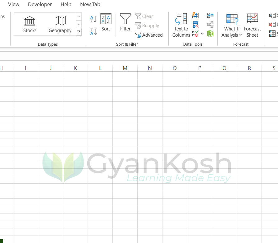
WHERE IS DATA VALIDATION OPTION OR BUTTON IN EXCEL 2013,2016,2019,2021 ?
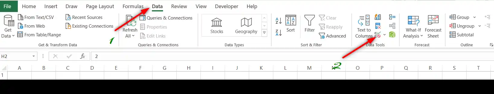
The data validation option can be found under the DATA TAB in the DATA TOOLS SECTION as shown in the picture below.
The following picture shows the location in Excel 2010,2013,2016,2019,2022, 365.
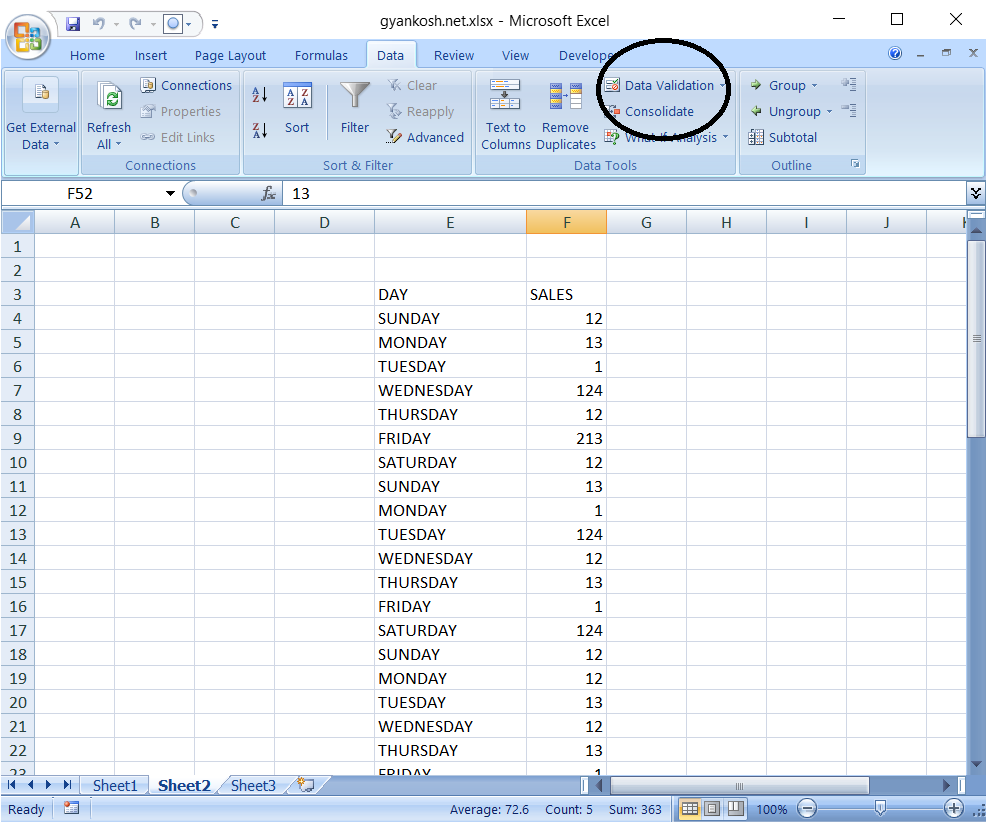
The following picture shows the data validation button location for Excel 2007.
EXAMPLE: USE DATA VALIDATION IN EXCEL
THE STEPS TO VALIDATE THE DATA HAVE BEEN DEMONSTRATED USING AN EXAMPLE.
SCENARIO:
Let us create a scenario where we need to enter the age and the age should be more than 18 and less than 30.
A cell containing the text “enter your age” is there. The next cell is the one to accept the input from the user.
STEPS:
- Click the cell where input is to be taken .
- Click CONDITIONAL FORMATTING button.Following dialog box will open.

PUTTING THE CONDITION IN PLACE:
The dialog box contains many conditions. We can choose the one we want.
For our example,
- we’ll choose ALLOW: WHOLE NUMBER. [As we want the age as whole numbers only ].
- DATA: BETWEEN and put the values as 18 for minimum and 30 for maximum as per the example statement.
ENTERING THE INPUT MESSAGE:
We have put the condition. But how would we tell our users about the condition?
Isn’t it the best idea to be able to show a comment when a particular cell is selected?
So, Excel provides us with this option which is very practical and helpful.
STEPS TO PUT THE INPUT MESSAGE IN DATA VALIDATION:
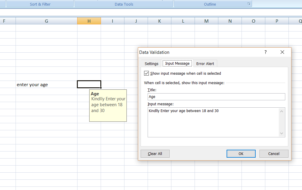
- Select the INPUT MESSAGE TAB in the DATA VALIDATION DIALOG BOX as shown in the picture below.
- Enter the title as per your requirement. We have entered AGE for our example.
- Enter the INPUT MESSAGE, the message which you want to show when the validated cell is selected by the user. For our example , we have put the message as KINDLY ENTER YOUR AGE BETWEEN 18 AND 30.
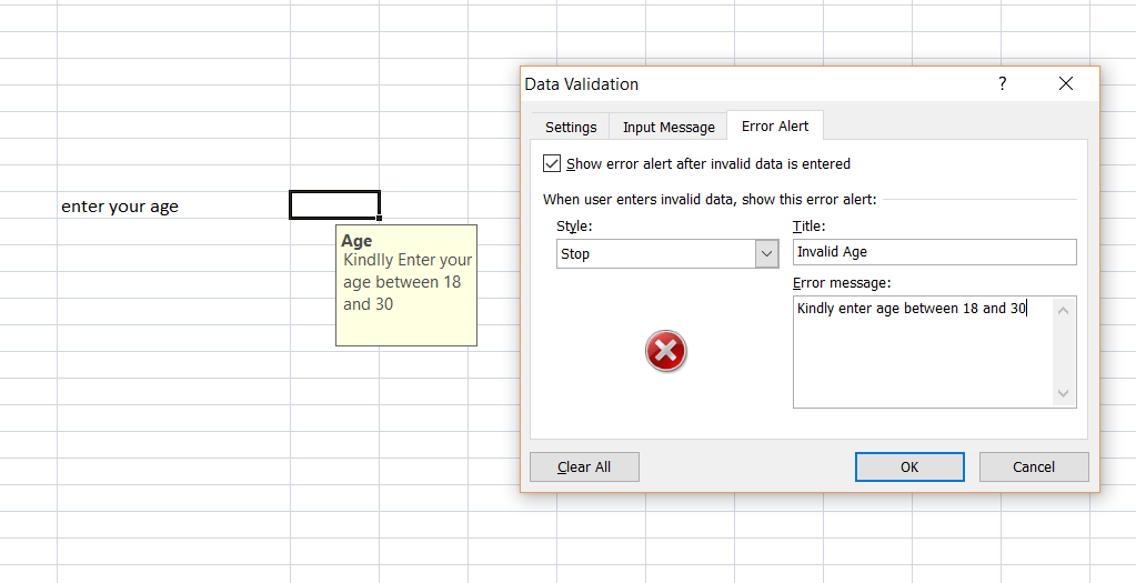
ENTERING THE ERROR ALERT MESSAGE:
In addition to the INPUT MESSAGE, we can put ERROR ALERT also.
STEPS TO ENTER ERROR ALERT:
- Choose the ERROR ALERT TAB in the DATA VALIDATION DIALOG BOX.
- Check the SHOW ERROR ALERT AFTER INVALID DATA IS ENTERED.
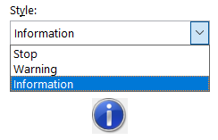
- Choose the Style from INFORMATION, STOP OR WARNING.
- Enter the title. For our example we have entered INVALID AGE.
- Enter the ERROR MESSAGE. For our example we have entered, KINDLY ENTER AGE BETWEEN 18 AND 30.
After all the settings are done, click OK.
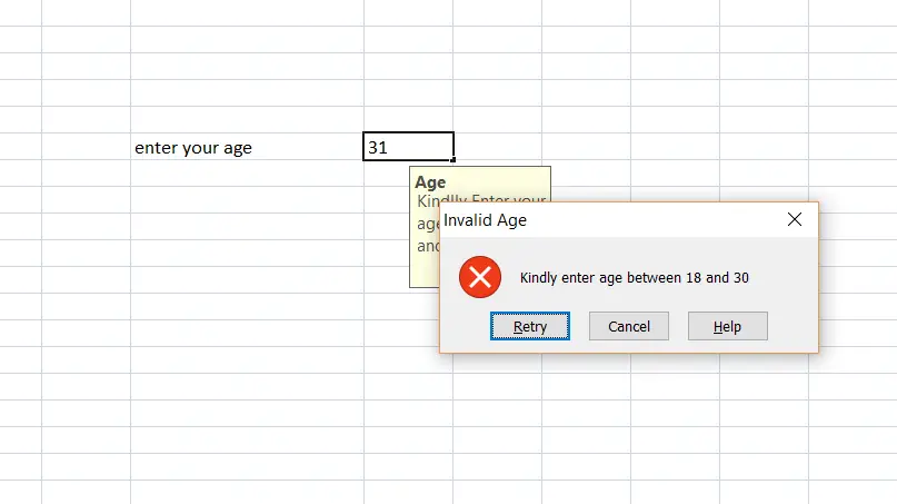
RUNNING THE EXAMPLE
After all the settings, we are ready to check our data validation.
For testing purposes, we put 31 and the cell didn’t accept the value and showed the error as we set
VALIDATE ALREADY FILLED DATA USING DATA VALIDATION
DATA VALIDATION provides us with a very useful functionality using which we can validate the data which is already present.
We have two options for validating already filled data.
- CIRCLE INVALID DATA
- CLEAR VALIDATION CIRCLES

Let us try these options using some random data.
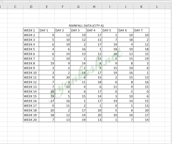
EXAMPLE:
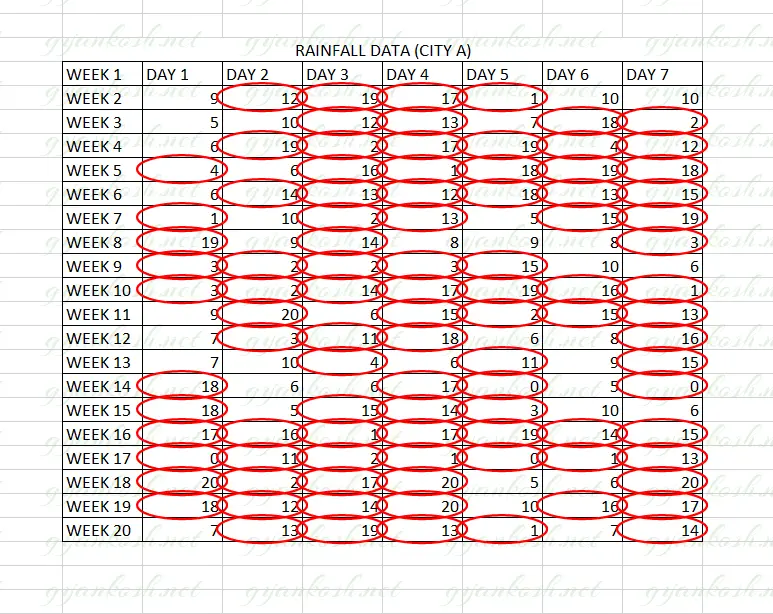
Let us take the rainfall data of a city for twenty week
Suppose we want to highlight the data when the rainfall was between 5 and 10.
The data is shown below.
STEPS TO HIGHLIGHT INVALID DATA
STEPS TO HIGHLIGHT INVALID DATA :
- Select the cells containing the rainfall data.
Go to DATA TAB> DATA VALIDATION DROP DOWN > DATA VALIDATION.
It’ll take us to the standard data validation dialog box.
Choose the options as shown in the animated picture below.
Make the selections as - ALLOW: WHOLE NUMBER
- DATA: BETWEEN
MINIMUM : 5
MAXIMUM:10 [ minimum and maximum fields will appear as soon as we choose DATA as BETWEEN ].
Now , again go to DATA TAB> DATA VALIDATION DROP DOWN > CIRCLE INVALID DATA.
As soon as we make the choice, all the invalid data will be encircled.
Look at the picture below for the reference.
The final picture shows the encircled data.
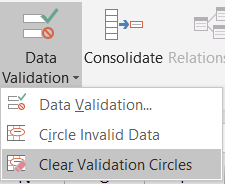
REMOVING DATA VALIDATION IN EXCEL
If we have circled the invalid data, we can easily clear these circles using the CLEAR VALIDATION CIRCLES under the DATA VALIDATION DROP DOWN LIST in DATA TAB.
FAQs
I CAN’T ENTER THE VALUES IN THE CELLS OF EXCEL SHEET?
It is quite possible that the cells are validated using DATA VALIDATION. Try removing the data validation.
IS DATA VALIDATION AVAILABLE IN EXCEL 365 ONLINE?
Yes, data validation is available. It can be found under the DATA TAB> DATA TOOLS which is the same location as found in the other versions of Excel.
WHAT IS SOURCE IN DATA VALIDATION IN EXCEL?
While creating a list in data validation, we get this field known as SOURCE.
SOURCE simply means the cells which contain the data to be enlisted in the dropdown.
HOW TO ADD CUSTOM WARNING MESSAGE IN DATA VALIDATION?
When we have put the conditions, we’ll need to convey this information to the user. You can visit here to learn the way to put WARNING MESSAGE.
HOW DO I USE EXCEL’S DATA VALIDATION TO DISPLAY COMMENTS OR DATA ENTRY TIPS?
Comments can be added separately in the cells, but yes, we can make use of the DATA VALIDATION too, to warn or inform the user about any information before he makes any changes to the cell.
It can be done by simply applying the INPUT MESSAGE as discussed here.
The INPUT MESSAGE will pop up, when you select the cell and are about to enter the data.
HOW TO APPLY DATA VALIDATION TO WHOLE COLUMN?
Simply select the complete column by clicking on the COLUMN name and after selecting the column, apply DATA VALIDATION.
This will apply the data validation to the entire column. You can also select the cells on which you want to apply data validation.
HOW TO REMOVE DATA VALIDATION FROM A COLUMN?
You can simply remove data validation by following steps:
- Select the column by clicking the COLUMN NAME.
- Go to DATA TAB> DATA VALIDATION.
- The DATA VALIDATION windows will open.
- Choose ANY VALUE in ALLOW DROP DOWN.
- The DATA VALIDATION is removed.
HOW TO APPLY DATA VALIDATION ON MULTIPLE COLUMNS?
We can simply apply data validation on multiple columns if we apply the data validation after selecting the multiple columns.
Follow the steps to apply data validation on multiple columns:
- Press and hold CTRL KEY on the keyboard.
- Click the COLUMN NAMES which you want to select.
- Don’t release the CTRL KEY until you are done.
- After all the columns have been selected , choose DATA VALIDATION option.
DATA VALIDATION WILL BE APPLIED TO ALL THE SELECTED CELLS.
HOW TO APPLY DATA VALIDATION ON MULTIPLE CELLS?
We can simply apply data validation on multiple cells if we apply the data validation after selecting the multiple cells.
Follow the steps to apply data validation on multiple columns:
- Press and hold CTRL KEY on the keyboard.
- Select the cell or range which you want to select.
- Don’t release the CTRL KEY until you are done.
- After all the columns have been selected , choose DATA VALIDATION option.
DATA VALIDATION WILL BE APPLIED TO ALL THE SELECTED CELLS.