Table of Contents
- PURPOSE OF TRANSPOSE FUNCTION IN EXCEL
- PREREQUISITES TO LEARN TRANSPOSE FUNCTION
- SYNTAX: TRANSPOSE FUNCTION IN EXCEL
- EXAMPLE 1:TRANSPOSE FUNCTION IN EXCEL: ARRAY
- EXAMPLE 2:TRANSPOSE FUNCTION IN EXCEL: A TABLE
- CONFUSION CLARIFICATIONS
Suppose we have a data which needs to be rotated i.e. the rows should become the columns and vice versa. How would we do that?
One method is , to create a new sheet and start doing this manually but would that be an efficient solution. What if the report is too big like 1000 lines or so.
The solution to this problem is the TRANSPOSE FUNCTIONS.
If you remember matrices, we used to find out the transpose of the matrix. We do the same here with the data.
TRANSPOSE FUNCTION comes under the LOOKUP AND REFERENCE group of functions in Excel.
TRANSPOSE FUNCTION converts the ROWS INTO COLUMN AND COLUMN INTO ROWS ( CALLED TRANSPOSE )
The transposing of data is many times required where we need to change the layout of the data for any reason.
The transposing can also be done by COPYING THE DATA, AND PASTING SPECIAL AND CHOOSING THE TRANSPOSE FUNCTION but that’ll create an additional copy of the data.[ Procedure discussed separately ]
PURPOSE OF TRANSPOSE FUNCTION IN EXCEL
TRANSPOSE FUNCTION rotates the layout of the data i.e. rows becomes the columns and columns becomes the rows. Simply stating it swaps rows and columns.
Transposing is needed sometimes due to the layout issues or some other reasons. It is not practical to do this process manually as the report may contain thousands of cells. So this method is very helpful in such cases.
PREREQUISITES TO LEARN TRANSPOSE FUNCTION
THERE ARE A FEW PREREQUISITES WHICH WILL ENABLE YOU TO UNDERSTAND THIS FUNCTION IN A BETTER WAY.
- Basic understanding of how to use a formula or function.
- Basic understanding of rows and columns in Excel.
- Of course, Excel software.
Helpful links for the prerequisites mentioned above What Excel does? How to use formula in Excel?
SYNTAX: TRANSPOSE FUNCTION IN EXCEL
The syntax ( the way how formula is phrased for excel) of MATCH is
=TRANSPOSE(ARRAY OF CELLS)
ARRAY ARRAY IS A GROUP OF CELLS WHICH CAN BE DECLARED AS A RANGE . ARRAY can be like A1:A10 OR A1:C10 with three columns and ten rows.or{1;2;3;4}
EXAMPLE 1:TRANSPOSE FUNCTION IN EXCEL: ARRAY
DATA SAMPLE
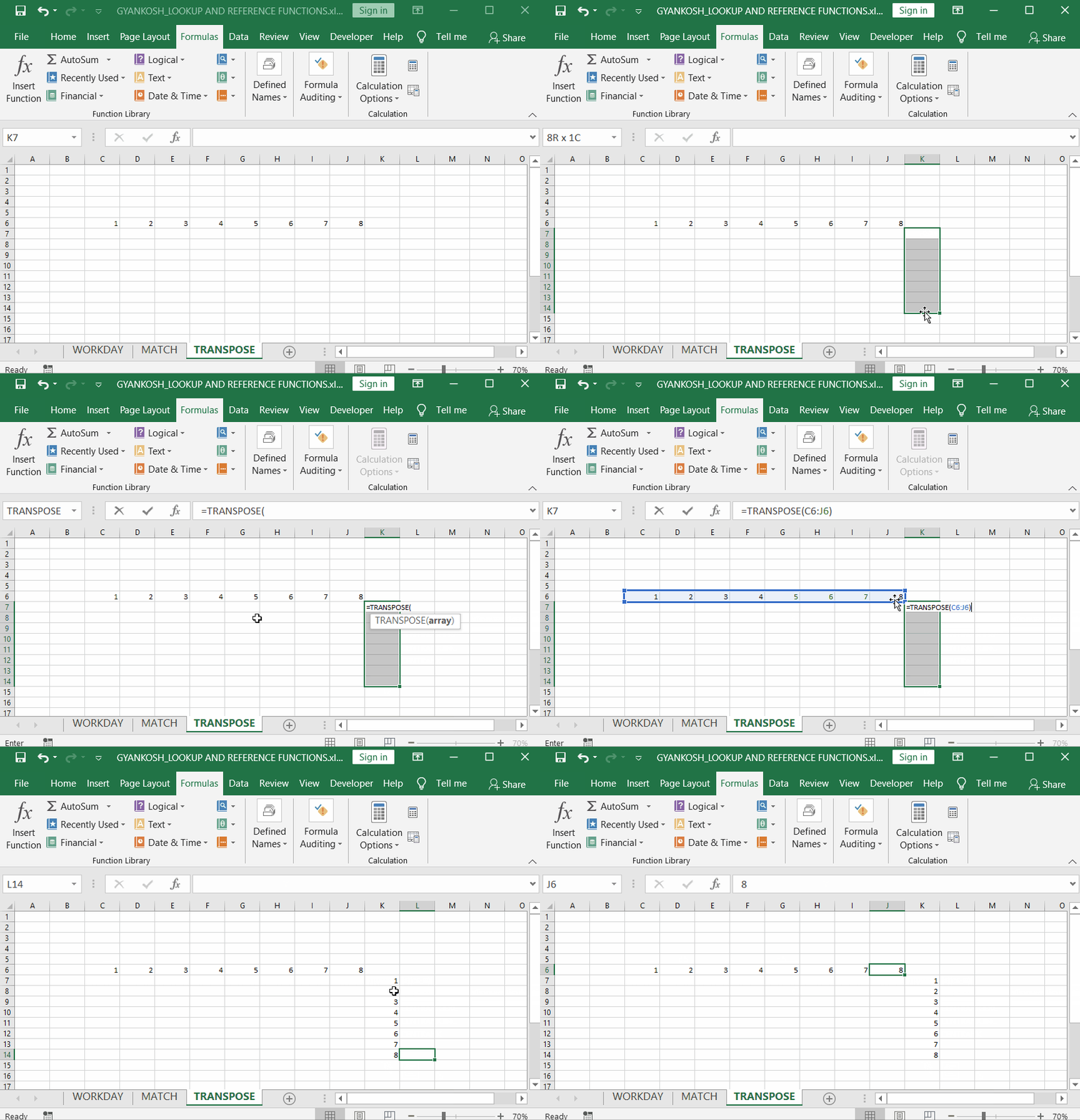
Let us try to transpose an array.Suppose the following array is present horizontally. 1 2 3 4 5 6 7 8We will transpose this array using the TRANSPOSE function.

STEPS TO APPLY TRANSPOSE FUNCTION
STEPS FOR THE EXAMPLE TAKEN If the array to be rotated from horizontal to vertical as discussed in example.
1. Select the exact number of cells in the same layout of the actual data which needs to be transposed i.e. with the same number of rows to be converted to same number of columns at a new place. Look at the picture above. We selected the exact 8 vertical cells before applying the function.
(K7 TO K14 in this case)
2. Now type the formula =TRANSPOSE(C6:J6) but don’t PRESS ENTER.
3. Press CTRL+SHIFT+ENTER.
4. The selected ARRAY will be transposed.
EXAMPLE 2:TRANSPOSE FUNCTION IN EXCEL: A TABLE
DATA SAMPLE
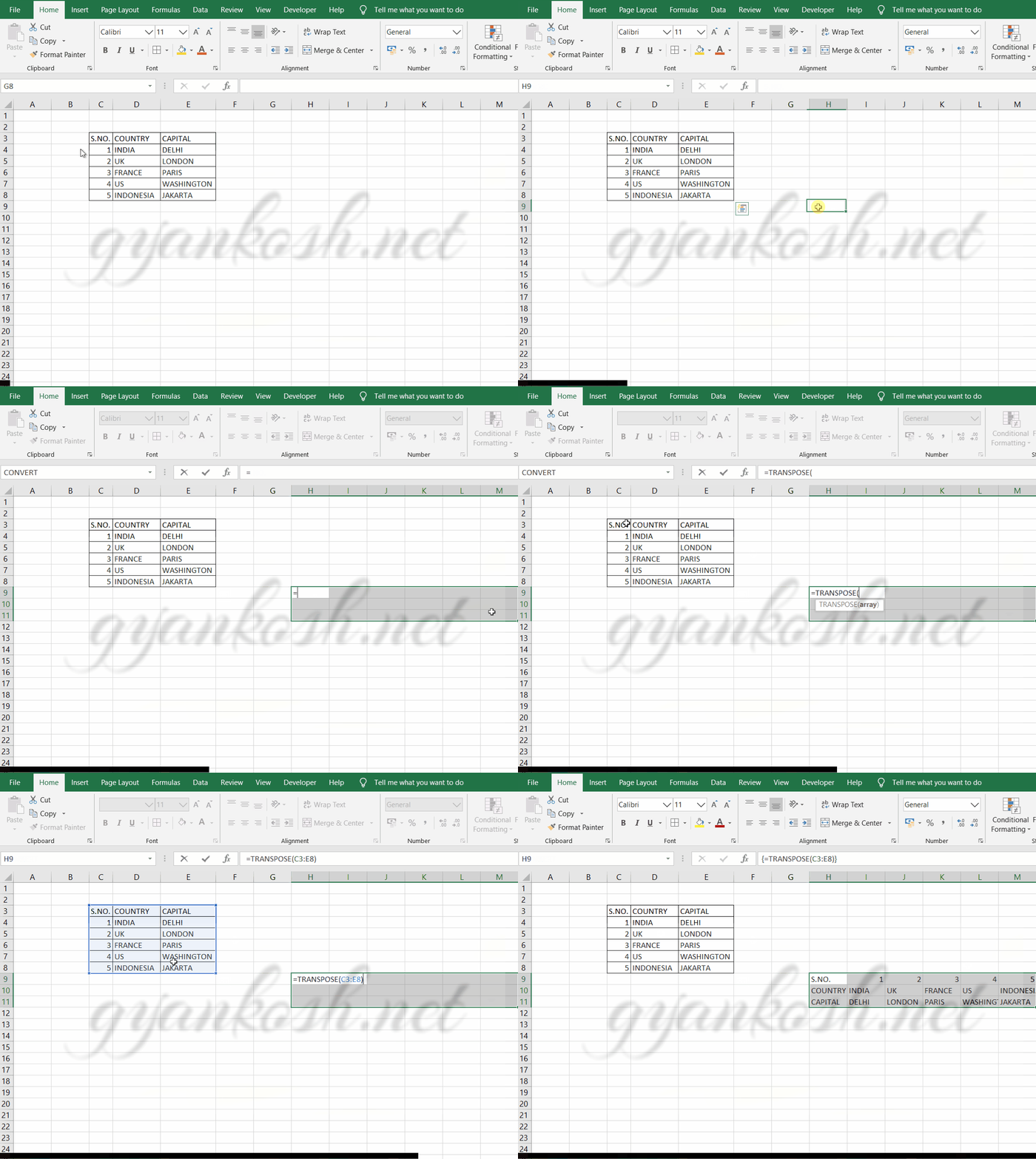
In previous example, we used the transpose function only on a single array. Now we’ll try it on a table.Let us try to transpose the following table.Suppose the following TABLE is present
| S.NO. | COUNTRY | CAPITAL |
| 1 | INDIA | DELHI |
| 2 | UK | LONDON |
| 3 | FRANCE | PARIS |
| 4 | US | WASHINGTON |
| 5 | INDONESIA | JAKARTA |
We will transpose this array using the TRANSPOSE function.

STEPS TO APPLY TRANSPOSE FUNCTION [EXAMPLE 2]
STEPS FOR THE EXAMPLE TAKEN Follow the following steps to rotate the table in EXCEL.REFER PICTURE: ABOVE 1. Check the number of rows and columns of the given table. e.g. our example table has 3 columns and 6 rows. Now select the layout for the transposed table i.e. 3 rows and 6 columns. Now do nothing, and start typing the formula starting with an “=”. The selection won’t be removed.2. Now type the formula =TRANSPOSE(C3:E8) but don’t PRESS ENTER.3. Press CTRL+SHIFT+ENTER.4. The selected table will be rotated [transposed]
If the array or a table is to be rotated from horizontal to vertical or vertical to horizontal as discussed in example.1. Select the exact number of cells in the same layout of the actual data which needs to be transposed i.e. with the same number of rows to be converted to same number of columns at a new place. 2. Now type the formula =TRANSPOSE(range of cells containing the data) but don’t PRESS ENTER.3. Press CTRL+SHIFT+ENTER.4. The selected ARRAY or TABLE will be rotated or transposed.
DO YOU KNOW??
IF WE PRESS ENTER DIRECTLY AFTER TYPING THE TRANSPOSE FUNCTION, THE ANSWER WILL NOT BE AS PER EXPECTATIONS. PRESS CTRL+SHIFT+ENTER.
CONFUSION CLARIFICATIONS
SELECTION BEFORE USING TRANSPOSE FUNCTION
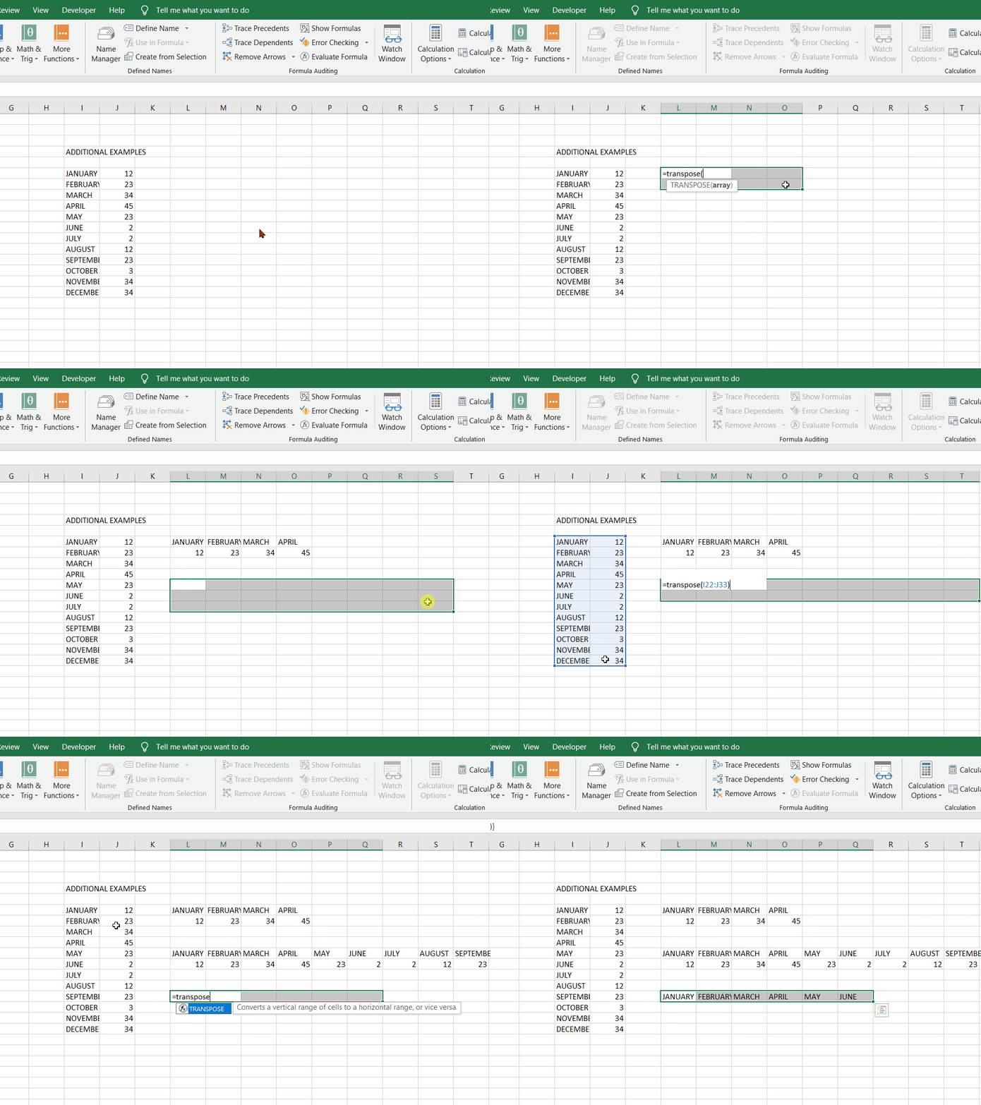
Selecting the cells before the usage of TRANSPOSE FUNCTION is very important. Let us check what will happen if the format is not exactly matching to the original cells.
The pre-selection of the cells (where we intend to transpose the original set of data) behaves like a mask.
e.g.
Suppose we have some data which shows the sales of cars in different months.
Now , we will try to transpose this data with different pre-selected cells.

