INTRODUCTION
IFERROR function comes under the LOGICAL FUNCTIONS category in Excel.
IFERROR is again a very useful function in excel which will be used a lot.
IFERROR returns the value of the formula if there is no error and other value if there is error.
IFERROR FUNCTON is a kind of error management system for the formulas and functions which we use in Excel. In programming we have a totally separate object for catching the errors. So we can compare the function to that ERROR OBJECT.
Suppose, we have a function which can have some undefined state (VALUE NOT AVAILABLE, N/A ETC. ), which, if not managed, would result in an error and can ruin our EXCEL APPLICATION. There are a few options to manage this situation. Either we need to enlist all such conditions and save our application from those conditions by introducing more complex functions or we can make the use of this great function.
In this article we’ll learn how IFERROR FUNCTION works , its syntax, usage and a few practical examples.
PURPOSE OF IFERROR IN EXCEL
IFERROR FUNCTION RETURNS THE VALUE OF THE FORMULA (IF IT GETS EVALUATED PROPERLY), OTHERWISE IT RETURNS THE SPECIFIED VALUE OR MESSAGE.
It is used to handle our functions which can return an error. e.g.
IFERROR( if function is evaluated properly, if function returns an error)
PREREQUISITES TO LEARN IFERROR
THERE ARE A FEW PREREQUISITES WHICH WILL ENABLE YOU TO UNDERSTAND THIS FUNCTION IN A BETTER WAY.
- Basic understanding of how to use a formula or function.
- Basic understanding of rows and columns in Excel.
- Of course, Excel software.
Helpful links for the prerequisites mentioned above
What Excel does? How to use formula in Excel?
SYNTAX: IFERROR FUNCTION
The Syntax for the function is
=IFERROR(EXPRESSION TO BE EVALUATED , VALUE IF ERROR)
EXPRESSION TO BE EVALUATED = THE FORMULA WHICH WE WANT TO EVALUATE.
VALUE IF ERROR= VALUE IF FORMULA GENERATES ANY ERROR
Few types of error being acted upon by the function are
#N/A, #VALUE!, #REF!, #DIV/0!, #NUM!, #NAME?, or #NULL!.
EXAMPLE: IFERROR FUNCTION IN EXCEL
DATA SAMPLE
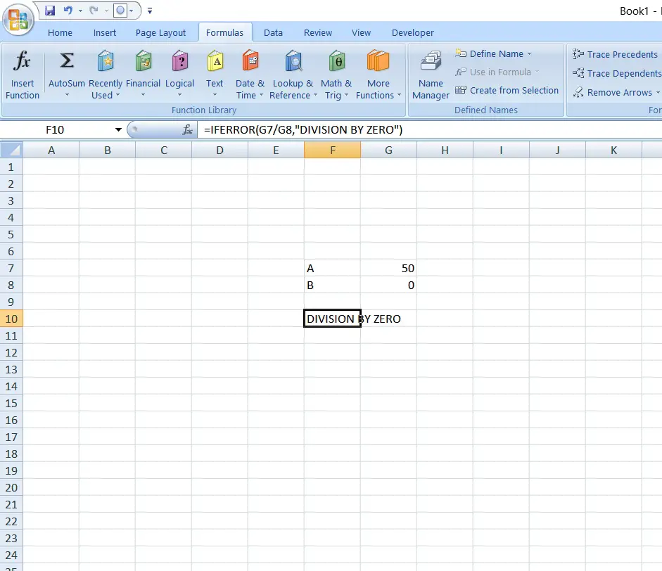
The simplest example can be a division by zero.Suppose there are two numbersA=50AND B=0We’ll be trying to evaluate A/B and if error occurs we’ll display a message “DIVISION BY ZERO”.

STEPS TO USE IFERROR
- We have A and B with values 50 and 0.
- We will evaluate A/B and put error message as “DIVISION BY ZERO”.
- The formula to be used is
- =IFERROR(G7/G8,”DIVISION BY ZERO”)
- The output is shown in the picture.
- The function evaluates A/B and finds the error DIV BY 0 and results in the message.
EXPLANATION
We have used the formula as
=IFERROR(G7/G8,”DIVISION BY ZERO”)
The first argument is the calculation which we want to perform i.e. G7/G8 .
The second argument is the message which we want to give if the first argument formula results in an error. Here we have used the text “Division by zero” . As the formula evaluates to an error, the message is displayed.
KNOWLEDGE BYTES
SOME FACTS ABOUT IFERROR
IFERROR can be used anywhere , where there are situations of generating errors.Simply put the formula in the first condition and error message or value in the second one. Standard way of catching an error=IFERROR(FORMULA TO BE EVALUATED, ANY VALUE OR MESSAGE [if the formula fails] ). FEW MORE POINTS TO REMEMBER:
- IFERROR only recognizes the error, but not the type of the error.
- IFERROR can be utilized cleverly to show the common value when no condition is met.
- IFERROR can not be nested as there is no further investigation possible into the error.