HOW TO SORT PIVOT TABLE IN GOOGLE SHEETS?

Table of Contents

• WHY AM I NOT ABLE TO SORT MY PIVOT TABLE IN GOOGLE SHEETS?
• STANDARD WAYS TO SORT PIVOT TABLE IN GOOGLE SHEETS

In this article, we’d learn the ways to sort pivot table in Google Sheets.

PIVOT TABLE is a very powerful tool which help us to create and check various operations on our table in multiple ways.

We call them PIVOT TABLE because of the flexibility to lay any data as a column or row within seconds and apply operation on them without affecting the reliability of the data.

Many times, we need to apply many operations on our pivot table. Sorting is one of the very basic operation which we might need to apply on our data.

Sorting is a simple arrangement of our data in a particular fashion say alphabetical or ascending or descending order. It help us to see any trend or makes the search of the data easier.

LEARN TO CREATE PIVOT TABLES HERE.

WHY AM I NOT ABLE TO SORT MY PIVOT TABLE IN GOOGLE SHEETS?

Sorting a pivot table is not handled by the standard sort option in Google Sheets. That’s the reason you are not able to use the standard way to sort your data.

If we use the standard sort option to arrange data in Pivot table of google sheets, it won’t get sorted and come back to the original form. We discuss the way to sort it in the following section.

STANDARD WAYS TO SORT PIVOT TABLE IN GOOGLE SHEETS

We can sort PIVOT TABLE easily using the following way.

We’ll start with the help of an example.

Let us take a simple data of rainfall in Cities A, B …. G for 6 months from January to June.

The data layout is shown in the picture below.

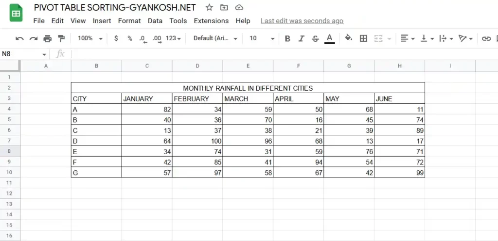
We’ll be sorting the cities with respect to the least to highest average rainfall in six months with the help of pivot table.

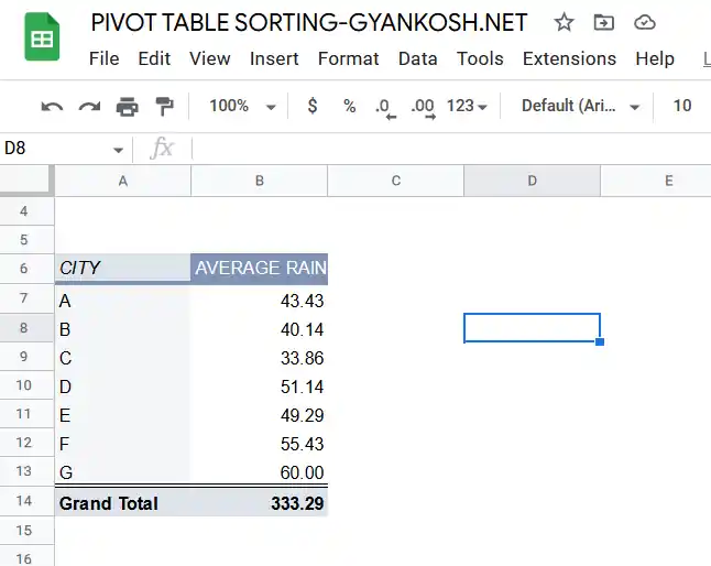
We’ll create a pivot table for this data with the use of City and Average Rainfall of six months columns as shown in the picture below.

LEARN CREATING PIVOT TABLE IN GOOGLE SHEETS HERE.

LEARN TO INSERT A CALCULATED FIELD IN GOOGLE SHEETS HERE.

1. Our pivot table will look something like the one shown below.

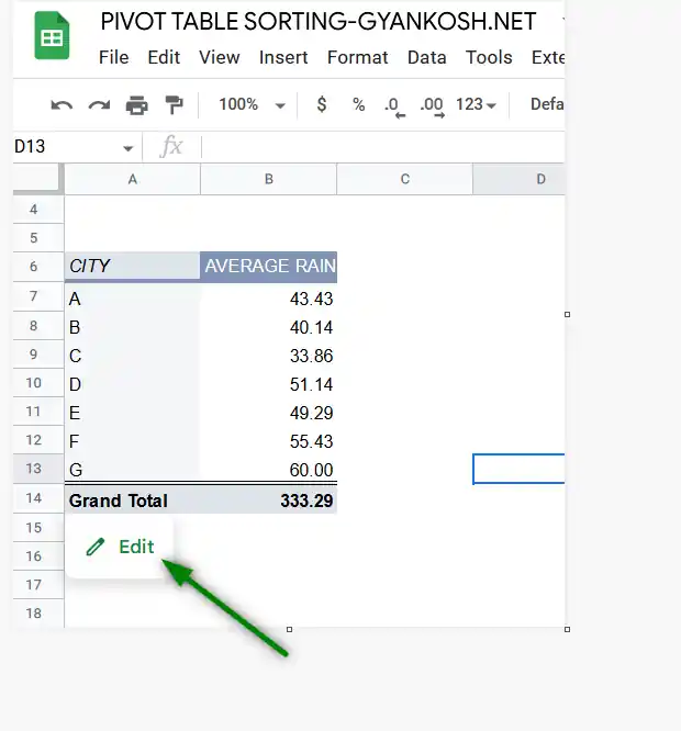
2. After the pivot table is ready [ which can be ready to use in your case ], hover the mouse over the pivot table or click anywhere on pivot table.
3. EDIT option will popup as shown in the picture below.
4. Click EDIT option.

As we click EDIT, PIVOT TABLE EDITOR window will appear on the right portion of the screen.

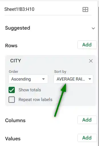
Go to ROWS or COLUMNS , whichever basis you want to sort your date as shown in the picture below.

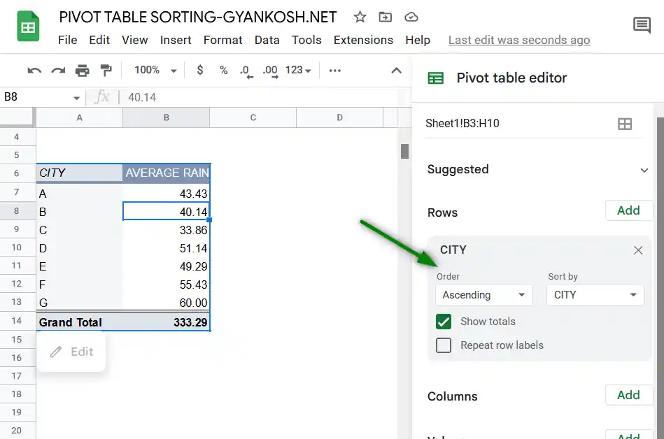
For our example, we want to sort the data on the basis of the AVERAGE RAIN COLUMN. [ Learn changing the column name of pivot table here ]

Select the ORDER, ASCENDING [ Smaller to larger ], or DESCENDING [ larger to smaller ].

Select the column for the SORT REFERENCE.

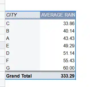
As soon as we make the selections, the data will be sorted as per the choices made.

The selections are shown below in the picture.

The final sorted pivot table is shown in the picture below.

So, we learnt the way to sort pivot table in google sheets.

Learn other Google Sheets tricks here.