Table of Contents
- INTRODUCTION
- PURPOSE OF INDIRECT FUNCTION IN GOOGLE SHEETS
- PREREQUISITES TO LEARN TRANSPOSE FUNCTION
- SYNTAX: INDIRECT FUNCTION IN GOOGLE SHEETS
- EXAMPLE 1: USE INDIRECT FUNCTION TO GET THE DATA IN THE CELL A1
- EXAMPLE 2: GET THE DATA IN THE CELL A1 WHEN THE ADDRESS IS IN ANOTHER CELL
- EXAMPLE 2: GET THE DATA IN THE CELL A1 USING THE RC NOTATION
INTRODUCTION
The functions are a very powerful tool present in the spreadsheet applications like GOOGLE SHEETS to solve many challenging problems.
The functions are self-contained entity that receives the variables and returns the output as per the type of the function.
Every function is apt to be used in a particular situation.
A situation can arise when we need to use an address that is already present in any cell or as a textual statement.
For such a situation we have got a function called INDIRECT in google sheets.
In this article, we’ll learn everything from the introduction, purpose, examples, and the usage of the Indirect function in Google Sheets.
PURPOSE OF INDIRECT FUNCTION IN GOOGLE SHEETS
INDIRECT FUNCTION RETURNS THE CELL REFERENCE GIVEN BY ANY STRING PASSED INTO THIS FUNCTION.
It simply means that we can enter any cell address as a TEXT as an argument and the function will point towards the address passed as a text.
This simple function is very useful and helps us to perform difficult procedures in Google Sheets.
Some of the situations where we can make use of INDIRECT FUNCTION can be
- When the cell address is present as the text.
- To pass any address as a text.
- To use the dropdown and choose the address which will depend on the selected text.
- Choose any values which are present in the different cells which can be chosen by using an indirect function.
- Can be used to use the R1C1 notation in google sheets.
and many other conditions.
PREREQUISITES TO LEARN TRANSPOSE FUNCTION
THERE ARE A FEW PREREQUISITES THAT WILL ENABLE YOU TO UNDERSTAND THIS FUNCTION IN A BETTER WAY.
- Basic understanding of how to use a formula or function.
- Basic understanding of rows and columns in GOOGLE SHEETS.
- Of course, Google Sheets login.
SYNTAX: INDIRECT FUNCTION IN GOOGLE SHEETS
The syntax ( the way how the formula is phrased for GOOGLE SHEETS) of INDIRECT FUNCTION is
=INDIRECT ( REFERENCE TO A CELL AS STRING, IF THE NOTATION IS A1)
REFERENCE TO A CELL AS STRING is simply the address of the cell as a string/text to which you want to refer.
IF THE NOTATION IS A1 If the reference is in the A1 style, choose TRUE if it is R1C1 style, choose FALSE.
If the second argument is skipped, it’ll be taken as A1 notation by default.
EXAMPLE 1: USE INDIRECT FUNCTION TO GET THE DATA IN THE CELL A1
DATA SAMPLE
For trying out our newly learned function INDIRECT , let us put some random data “WELCOME TO GYANKOSH.NET” in the cell A1.
In the solution, we’ll try to get this data using the INDIRECT FUNCTION bypassing the cell address as text and getting the reference from the other cell too.
The data is shown in the following picture.
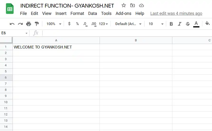
EXAMPLE DATA
Let us get the data in cell B6 using the indirect function.0
If we want to get the data directly in the B6, we’ll use the formula as =A1 and it’ll bring the data to B6 directly. But here, we want to use the function indirect.
So follow the steps to use the indirect function to get the data.
STEPS TO GET THE DATA IN A1 USING INDIRECT FUNCTION
- Simply double-click the cell where you want the result to get started.
- Enter the formula as =INDIRECT(“CELL ADDRESS”, TRUE [IF A1 NOTATION ])
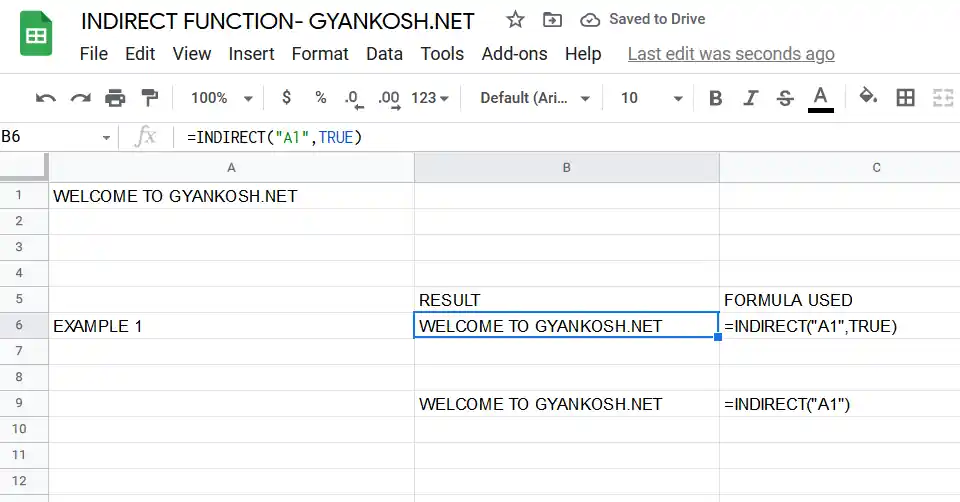
- For our example, we’ll enter the formula in the cell B6 as =INDIRECT(“A1”, TRUE)
- Press Enter.
- The result will appear in the cell. The result will be the text WELCOME TO GYANKOSH.NET which is actually present in cell A1.
In cell B9, we tried the same formula without using the second argument. As we know that, the value is taken as TRUE by default which is verified as the result is the same.
The formula used in the cell B9 is =INDIRECT(“A1”)
EXAMPLE 2: GET THE DATA IN THE CELL A1 WHEN THE ADDRESS IS IN ANOTHER CELL
DATA SAMPLE:
In this example, we already have the text WELCOME TO GYANKOSH.NET in the cell A1.
We have put the address A1 as text in cell C14.
We’ll use the indirect function to address cell A1 indirectly.
We will transpose this array using the TRANSPOSE function.
STEPS TO GET THE DATA IN A1 WHEN THE CELL ADDRESS IS KEPT IN THE CELL C14
- Simply double click the cell where you want the result to get started.
- Enter the formula as =INDIRECT(CELL ADDRESS CONTAINING THE ACTUAL LOCATION, TRUE [IF A1 NOTATION ])
- For our example, we’ll enter the formula in the cell B6 as =INDIRECT(C14,TRUE) [C14 CONTAINS THE TEXT “A1”]
- Press Enter.
- The result will appear as WELCOME TO GYANKOSH.NET
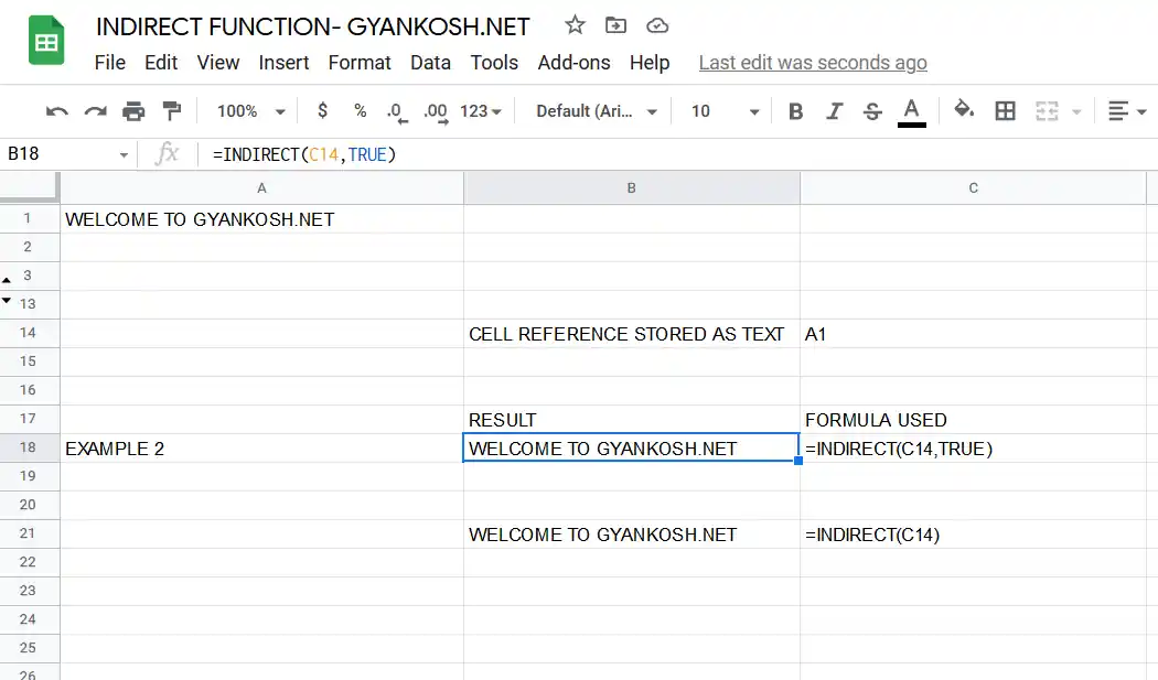
In cell B21, we tried the same formula without using the second argument. As we know, the value is taken as TRUE by default which is verified as the result is the same.
The formula used in cell B21 is =INDIRECT(C14).
EXAMPLE 2: GET THE DATA IN THE CELL A1 USING THE RC NOTATION
DATA SAMPLE:
In this example, we already have the text WELCOME TO GYANKOSH.NET in cell A1.
We have put the address A1 as text in cell C14.
We’ll use the indirect function to address the cell A1 indirectly.
We will transpose this array using the TRANSPOSE function.
STEPS TO GET THE DATA IN A1 WHEN THE CELL ADDRESS IS KEPT IN THE CELL C14
- Simply double click the cell where you want the result to get started.
- Enter the formula as =INDIRECT(CELL ADDRESS CONTAINING THE ACTUAL LOCATION, TRUE [IF A1 NOTATION ])
- For our example, we’ll enter the formula in the cell B6 as =INDIRECT(C14,TRUE) [C14 CONTAINS THE TEXT “A1”]
- Press Enter.
- The result will appear as WELCOME TO GYANKOSH.NET
In cell B21, we tried the same formula without using the second argument. As we know, the value is taken as TRUE by default which is verified as the result is the same.
The formula used in the cell B21 is =INDIRECT(C14).
