Table of Contents
- INTRODUCTION
- COMBINING INDEX AND MATCH IN GOOGLE SHEETS
- PURPOSE OF INDEX-MATCH IN GOOGLE SHEETS
- SYNTAX: INDEX-MATCH IN GOOGLE SHEETS
- EXAMPLE 1:HOW TO USE INDEX MATCH FOR LOOKUP IN GOOGLE SHEETS
- EXPLANATION:
- EXAMPLE 2: USING INDEX MATCH CLUBBED WITH OTHER FUNCTION
- CONFUSION CLARIFICATIONS
INTRODUCTION
INDEX-MATCH is the combination of two great functions INDEX and MATCH which are very useful in practical usage of Google Sheets.
This combination helps us to find out the values , corresponding to any lookup value from the same or another table within a fraction of seconds.
It becomes very important to learn these tricks in order to be efficient in GOOGLE SHEETS.
Let us first review both of these functions individually , so that we can understand how they would work in conjunction to make our lookup better and faster.
INDEX FUNCTION returns the value of a cell or array in a specified relative location given by row no. and column no. in a selected range.
Relative position is the position with respect to the select LOOKUP_RANGE.
e.g.
We have five COLORS and five CODES and we need to find out a value on a particular position.
So we can use INDEX function for this scenario and it’ll find out the item to be searched at a particular position.
Suppose there is a table of 4 columns and 4 rows.
If we want to search that what element is present at row no. 3 and column no. 4, we’ll take help of INDEX FUNCTION.
If you want to have an in depth understanding of INDEX FUNCTION by solving the examples.
MATCH FUNCTION looks up VALUE_TO_BE_FOUND in the given range and returns its relative position.
Relative position is the position with respect to the select LOOKUP_RANGE.
e.g.
We have five COLORS and five CODES and we need to find out at which position ,any specified color is present.
The lookup value will be color code, and the lookup range will be the range of colors.
The result will be the relative position of the color with respect to the selection.
If you want to have an in depth understanding of MATCH FUNCTION by solving the examples.
Now if you notice, both the functions are almost opposite to each other.
So it is possible to combine both of them to get better use of both the functions to lookup and retrieve the value from a big pool of data. Let us see how we can use them.
COMBINING INDEX AND MATCH IN GOOGLE SHEETS
Index and Match functions are opposite to each other.
Index function finds out the value of an item at a particular location in an array whereas Match function returns the relative position of an item after matching it from a given list.
So we can combine both the functions to retrieve the value from any column, against a lookup value which will be searched by the MATCH function for us. Let us try to put this in the form of a function.
Syntax is given in the next Section.
PURPOSE OF INDEX-MATCH IN GOOGLE SHEETS
Index Match create a very powerful pair to help us with one of the very important requirement of matching a value and extracting the other values corresponding to this matched one.
The combined INDEX-MATCH functions can be used to pull out any value which is corresponding to the another lookup value from another set of data which may or may not be on the same sheet.
SYNTAX: INDEX-MATCH IN GOOGLE SHEETS
Let us learn the way this function will be written in GOOGLE SHEETS.
The INDEX-MATCH FUNCTION will be used in the following format when used for lookup.
=INDEX( Array or TABLE from where the value is finally needed , MATCH(LOOKUP VALUE, Array in which the value will be found, match mode ), relative column number )
Array or Table from where the value is finally needed This is the table from which the value will be extracted finally
MATCH Lookup Value The unique value on the basis of which , we’ll find the desired value.
Array in which the value will be found This is the column where the value will be found
Match Mode Different match modes of MATCH FUNCTION.
Relative Column Number The column number of the INDEX (first argument) which will be returned for the value after the matching has been done.
EXAMPLE 1:HOW TO USE INDEX MATCH FOR LOOKUP IN GOOGLE SHEETS
We have a data sample with the students having different marks in different subjects. We’ll try a simple lookup of the data through index match first.
The data given is shown in the picture.
| STUDENTS | MATHEMATICS | SCIENCE | ARTS | LANGUAGE | SOCIAL SCIENCE |
| ASHU | 89 | 85 | 96 | 69 | 85 |
| DAVID | 85 | 96 | 95 | 67 | 54 |
| JOE | 96 | 56 | 82 | 83 | 87 |
| CREG | 85 | 89 | 98 | 69 | 67 |
| RAM | 75 | 79 | 78 | 91 | 58 |
| PETER | 96 | 78 | 94 | 97 | 96 |
We’ll try to find the student with 83 marks in LANGUAGE. After that we’ll find the person who got 67 marks too.
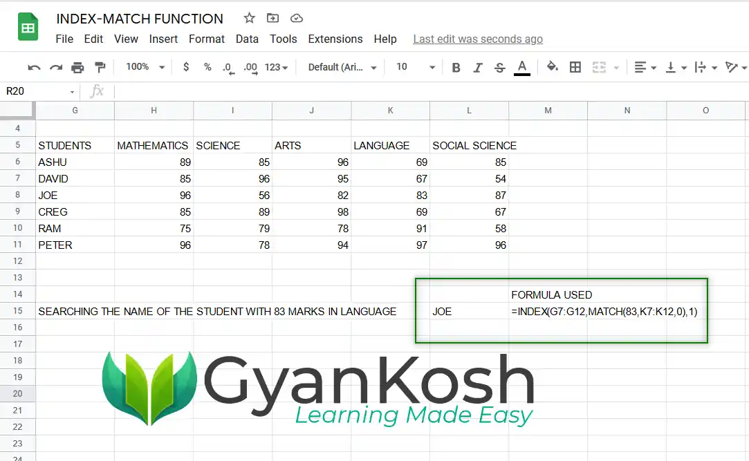
EXPLANATION:
We put the formula as
=INDEX(G7:G12,MATCH(83,K7:K12,0),1)
G7:G12 is the table from which we need the result. Right now we selected just the column from where we need the name.
Match started as it’d return us the index.
83 is the value to be found.
k7:k12 IS THE ARRAY WHERE 67 WILL BE COMPARED WITH.
0 IS THE EXACT MATCH
Third argument of INDEX function is the column number to return which is 1 as we have selected single column.
The result appears as JOE which is correct.
After this we change the lookup value as 67 and see that result changes to David.
EXAMPLE 2: USING INDEX MATCH CLUBBED WITH OTHER FUNCTION
DATA SAMPLE
Find out the students who has highest marks in Science.The data is given as the following table
| STUDENTS | MATHEMATICS | SCIENCE | ARTS | LANGUAGE | SOCIAL SCIENCE |
| ASHU | 89 | 85 | 96 | 69 | 85 |
| DAVID | 85 | 96 | 95 | 67 | 54 |
| JOE | 96 | 56 | 82 | 83 | 87 |
| CREG | 85 | 89 | 98 | 69 | 67 |
| RAM | 75 | 79 | 78 | 91 | 58 |
| PETER | 96 | 78 | 94 | 97 | 96 |
Let us try to find out the highest marks in Science.

EXPLANATION
We have to find the highest marks in Science.
For that we need to lookup for the highest marks first which we can do with the help of LARGE FUNCTION.
So we put it inside the Match Function.The function used to solve the problem is
=INDEX(G26:G31,MATCH(LARGE(I26:I31,1),I26:I31,0),1)
G26:G31 is the array from which we need the output.
Match function is started.
We’ll lookup the value which is highest for which we’ll use LARGE function.
I26:I31 is the array from which the value is to be matched.
0 is for the exact match.
1 in index function is for returning the value of the first column.
The answer is shown as DAVID which is correct.
CONFUSION CLARIFICATIONS
THE RELATIVE ROW AND COLUMN NUMBER
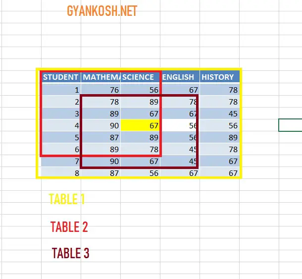
A cell is filled with YELLOW COLOR which we want to find. Now let us see in how many ways we can get this value.
The row and column number of the INDEX FUNCTION is relative to the RANGE SELECTED.
If we select Table 1, the value to be found will be at the row no. 4 and column no. 3.
If we select Table 2, the value to be found will be at the row no. 4 and column no. 3 again.
If we select Table 3, the value to be found will be at the row no. 3 and column no. 2.
So all these three different notations result in the same result. So always take care of the range selected and row and column no. selected.