Freezing panes (Certain Rows/Columns having headings etc.) in GOOGLE SHEETS is very important when we are working with big and lengthy reports .
In very large reports having many columns or rows, it becomes difficult to remember the column names and we are confused which is very irritating.
We need to scroll up the report over and again to remind us of the column or row headings.
It happens at the time of creating reports as well as when we are checking or reviewing them.
When the reports are sent to somebody, this problem emerges again.
So , our topic, freezing panes give us the solution to this very problem.
Even if we are creating the reports or we are studying them, it is always needed to know about the column or row headings otherwise it would be difficult In that case, freezing panes is very helpful as it fixes our Rows Headings or Column Headings sticking to our screen while the data can scroll up or down or left or right .
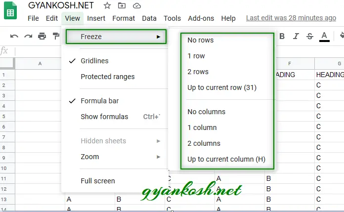
BUTTON LOCATION TO FREEZE ROWS IN GOOGLE SHEETS
FREEZE ROWS options are present under the VIEW MENU in GOOGLE SHEETS.
STEPS TO FREEZE TOP ONE OR TWO ROWS
Google Sheets has different options for freezing the top rows or left columns. We will discuss them one by one.
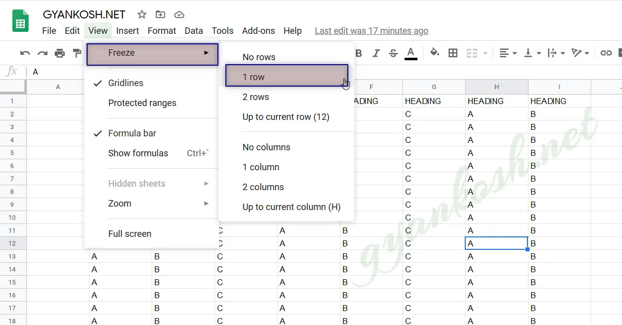
STEPS TO FREEZE TOP ONE ROW IN GOOGLE SHEETS:
- Go to VIEW MENU>FREEZE.
- Click the options 1 ROW
The TOP ROW of the sheet will be frozen.
Google Sheets has different options for freezing the top rows or left columns. We will discuss them one by one.
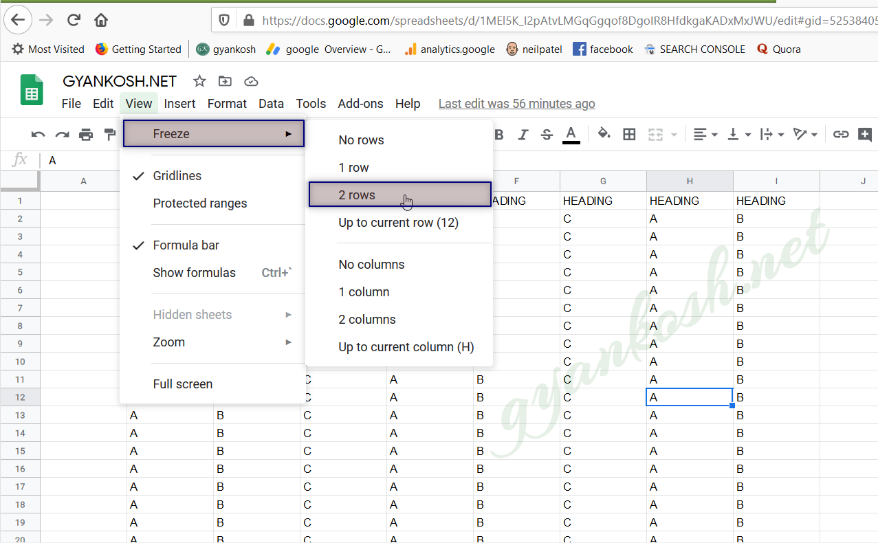
STEPS TO FREEZE TOP TWO ROWS IN GOOGLE SHEETS:
- Go to VIEW MENU>FREEZE.
- Click the options 2 ROW
The TOP TWO ROWS of the sheet will be frozen.
Google Sheets has different options for freezing the top rows or left columns. We will discuss them one by one.
STEPS TO FREEZE CUSTOM NUMBER OF ROWS IN GOOGLE SHEETS:
If we want to freeze the number of rows we want, follow the given steps.
- Select the row upto which you want to freeze the rows.
- Click VIEW MENU> FREEZE
- Click the options UPTO CURRENT ROW.
The rows including the SELECTED CELL will be frozen. The picture below shows the complete process of freezing the custom number of rows in google sheets.
STEPS TO FREEZE ONE OR TWO COLUMNS IN GOOGLE SHEETS
Google Sheets has different options for freezing the top rows or left columns. We will discuss them one by one.
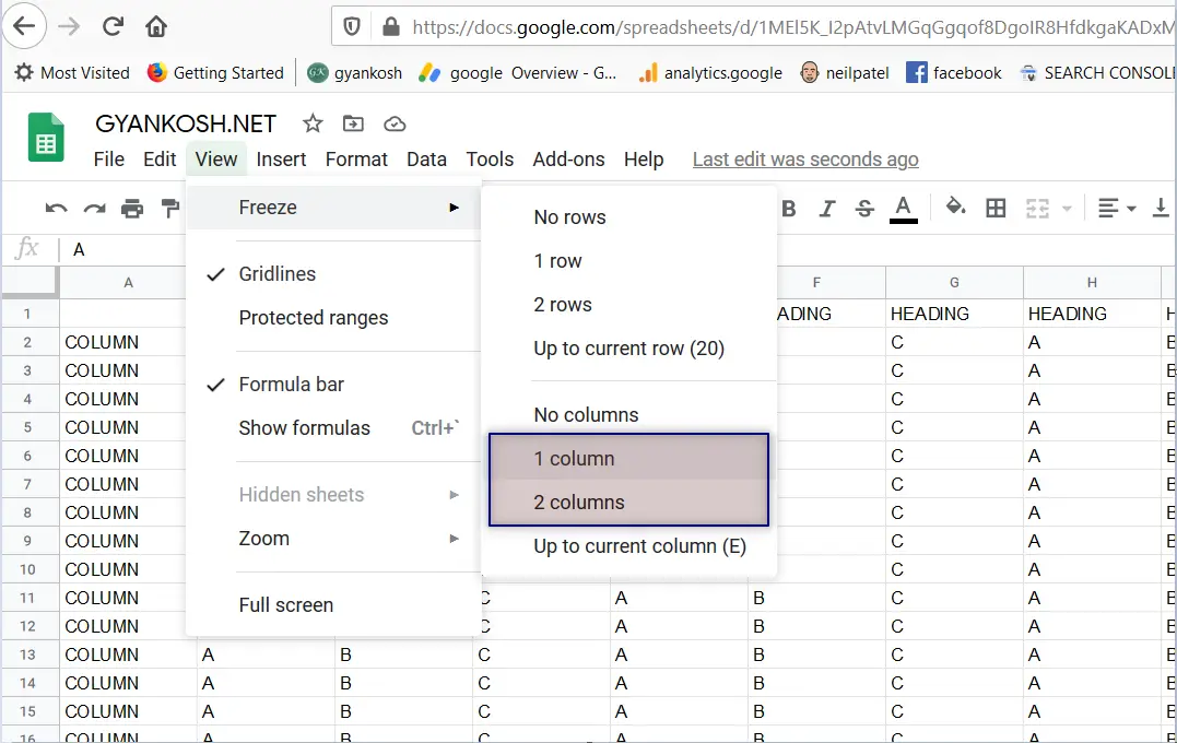
STEPS TO FREEZE LEFT ONE OR TWO COLUMNS IN GOOGLE SHEETS.
- Go to VIEW MENU>FREEZE.
- Click the options 1 COLUMN for freezing one column and 2 COLUMN for freezing two columns.
The LEFT ONE OR TWO COLUMNS of the sheet will be frozen.
Google Sheets has different options for freezing the top rows or left columns. We will discuss them one by one.
STEPS TO FREEZE CUSTOM NUMBER OF COLUMNS IN GOOGLE SHEETS:
If we want to freeze the number of rows we want, follow the given steps.
- Select the row up to which you want to freeze the columns.
- Click VIEW MENU> FREEZE
- Click the options UP TO CURRENT COLUMN.
The COLUMNS FROM THE FIRST UP TO the SELECTED CELL will be frozen. The picture below shows the complete process of freezing the custom number of COLUMNS in google sheets.
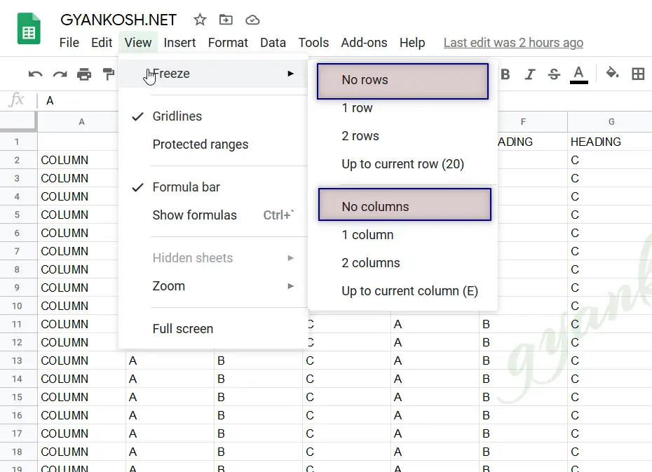
UNFREEZING ROWS OR COLUMNS IN GOOGLE SHEETS
UNFREEZE ROWS OR COLUMNS-If we want to unfreeze the rows or columns , we can follow the following steps.
- Go to VIEW MENU >FREEZE
- Choose NO ROWS.
- Choose NO COLUMNS.
After choosing both of the options all the freezing will be removed either it is present in the rows or columns.