HOW TO COPY OR DUPLICATE CONDITIONAL FORMATTING IN GOOGLE SHEETS?

Table of Contents

• INTRODUCTION
• DIFFERENT WAYS TO COPY CONDITIONAL FORMATTING IN GOOGLE SHEETS
• HIGHLIGHTING THE ATTENDANCE BETWEEN 90 AND 95 PERCENT
• 1. USING CONDITIONAL FORMATTING COPY OPTION
• STEPS TO COPY CONDITIONAL FORMATTING USING DIRECT PROVIDED OPTION
• 2. EDITING THE ” APPLY TO ” RANGE DIRECTLY TO COPY CONDITIONAL FORMATTING
• STEPS TO COPY CONDITIONAL FORMATTING BY EDITING THE APPLY TO RANGE
• FAQs
• HOW TO COPY CONDITIONAL FORMATTING FROM ONE SHEET TO ANOTHER ?
• FAQs
• SUGGESTED READS:

INTRODUCTION

To have the knowledge of Conditional formatting is very important if we want to apply GOOGLE SHEETS in our day to day jobs.

Conditional formatting is the  formatting [ font, color, fill color , size etc. ] of data as per its value of the content of the cells.

The ways of using CONDITIONAL FORMATTING in GOOGLE SHEETS is already discussed in the article

HOW TO USE CONDITIONAL FORMATTING IN GOOGLE SHEETS?. [ CLICK ANYWHERE ON THIS LINE TO VISIT THE ARTICLE ].

A situation may arise when we need  to simply copy the already applied conditional formatting rules for some new data.

For this situation , we’ll discuss various ways using which we can copy the conditional formatting rules easily from one data to other without affecting its efficacy.

DIFFERENT WAYS TO COPY CONDITIONAL FORMATTING IN GOOGLE SHEETS

YOU ARE SUPPOSED TO BE HAVING THE NECESSARY KNOWLEDGE ABOUT THE APPLICATION OF CONDITIONAL FORMATTING IN GOOGLE SHEETS

IF NOT CLICK HERE.

THE CONDITIONAL FORMATTING CAN BE COPIED DIRECTLY IN TWO WAYS

1. Using the CONDITIONAL FORMATTING COPY option.

2. Editing the  APPLY TO RANGE data directly.         

Let us take an example for learning the ways to copy conditional formatting.

EXAMPLE:

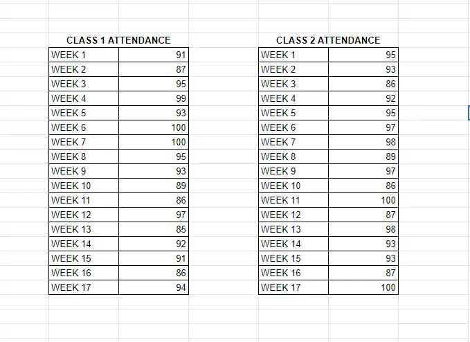
Let us take attendance of two different classes of students.

First column contains the WEEK NUMBER whereas second column contains the ATTENDANCE PERCENTAGE.

We’ll highlight the week when the attendance was between 90 to 95 percent in CLASS 1.

We’ll copy the CONDITIONAL FORMATTING rules for CLASS 2 directly using our two methods.

HIGHLIGHTING THE ATTENDANCE BETWEEN 90 AND 95 PERCENT

The first step is to apply the CONDITIONAL FORMATTING and highlight the Week with attendance percentage between 90 and 95.

STEPS TO APPLY CONDITIONAL FORMATTING ON THE DATA OF CLASS 1.

• Select the cells containing attendance cells of CLASS 1 i.e. only second column of the data.
• Go to FORMAT MENU and choose CONDITIONAL FORMATTING.
• The CONDITIONAL FORMATTING RULES box will open on the right.
•  The APPLY TO field will be filled already as we selected the range already.
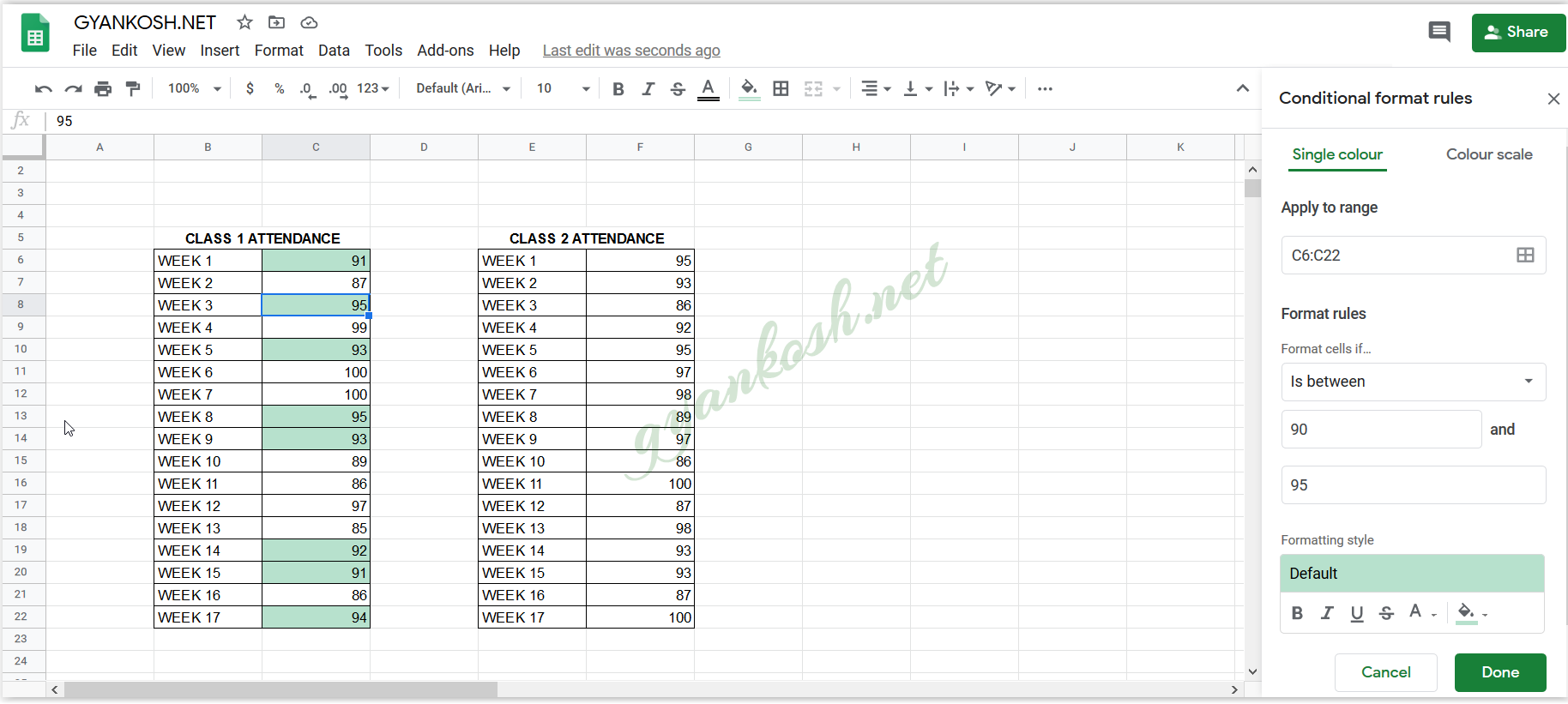
• Go to FORMULA RULES and choose IS BETWEEN from the drop down list.
• Enter the minimum value in the first field as 90 and 95 in the second field.
• Select the FORMATTING for the fill color as GREEN.
• Click DONE.
• All the week with attendance between 90 and 95 will be highlighted with a green color.
• [ THE ELABORATED PROCEDURE IS SHOWN IN THE LINK BELOW ]

The following picture shows all the settings.

CLICK HERE TO LEARN THE BASICS OF CONDITIONAL FORMATTING IN GOOGLE SHEETS.

After we have applied the conditional formatting in one of the tables. Let us try the different ways to copy the conditional formatting directly to the second table.

1. USING CONDITIONAL FORMATTING COPY OPTION

We have already applied conditional formatting to the data of CLASS 1 and highlighted all the attendance between 90 pc and 95 pc.

Now let us try to copy the conditional formatting directly to CLASS 2 without applying it individually to CLASS 2 using the standard lengthy process.

IN THIS EXAMPLE, WE ARE ONLY COPYING THE CONDITIONAL FORMATTING WHICH MEANS THAT THE ATTENDANCE BETWEEN 90 TO 95 PERCENT WILL BE HIGHLIGHTED.

STEPS TO COPY CONDITIONAL FORMATTING USING DIRECT PROVIDED OPTION

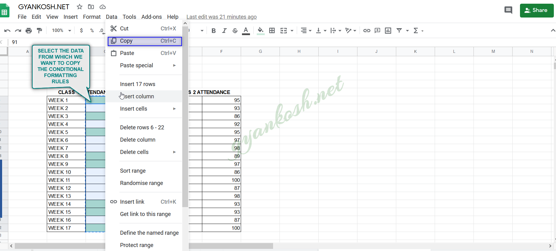
• Select all or any cell from the cells where the conditional formatting is applied. [ Conditional formatting rules which we want to copy ].
• Press CTRL+C or RIGHT CLICK> COPY.

The following picture depicts the process.

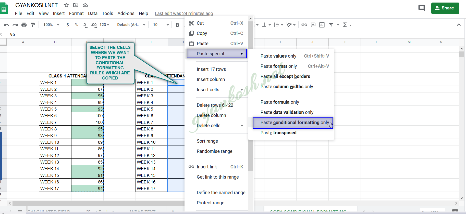
• Now, select all the cells where we want to apply the copied conditional formatting rules.
• RIGHT CLICK > Choose PASTE SPECIAL > PASTE CONDITIONAL FORMATTING ONLY.
• The conditional formatting will be applied to the selected cells.

The following picture depicts the process of pasting the conditional formatting.The following picture depicts the process.

The conditional formatting is applied to the new data as well.

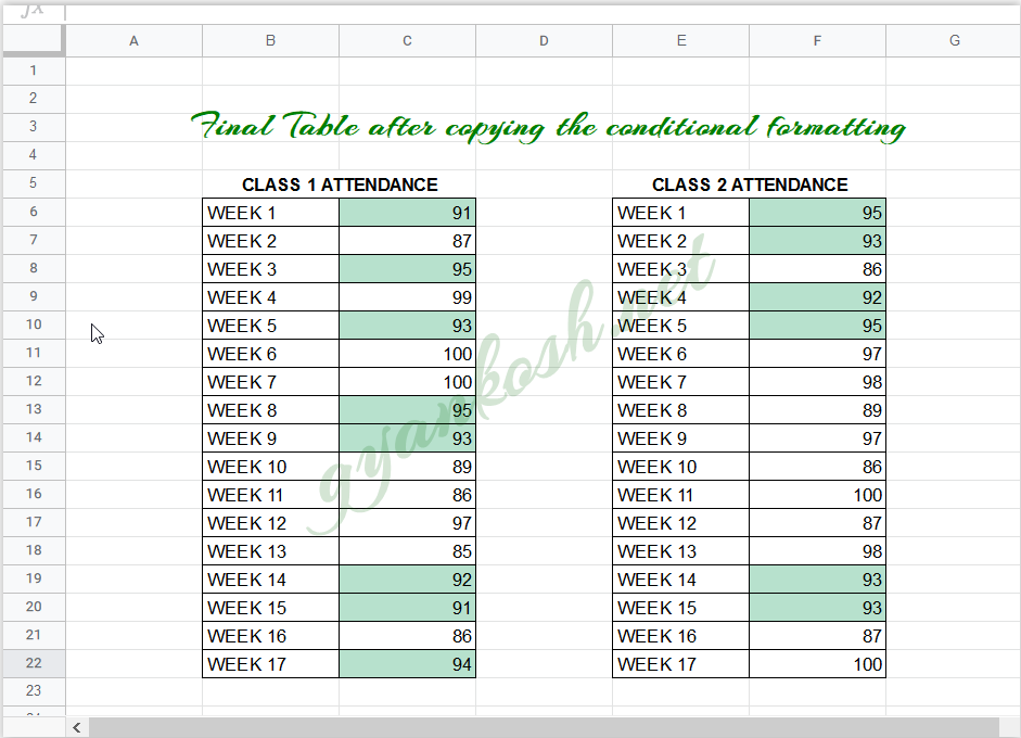
Final picture is shown below.

Pretty simple! Right ?

2. EDITING THE ” APPLY TO ” RANGE DIRECTLY TO COPY CONDITIONAL FORMATTING

After we have already copied the conditional formatting successfully using the direct pasting option , now let us try a simpler solution to the same problem. 

When we copy and paste the conditional formatting, it simply adds the Address of the Additional range in the format rules.

If we do that directly, we need not to copy and paste the conditional formatting from the cells. 

STEPS TO COPY CONDITIONAL FORMATTING BY EDITING THE APPLY TO RANGE

• Select any cell, from the range , on which the conditional formatting has been applied which we want to copy. [ Cell from the conditional formatting data which is to be copied ].
• If CONDITIONAL FORMATTING RULES box is not open, go to FORMAT MENU and choose CONDITIONAL FORMATTING.
• The Conditional Formatting Rules option box will open.
  

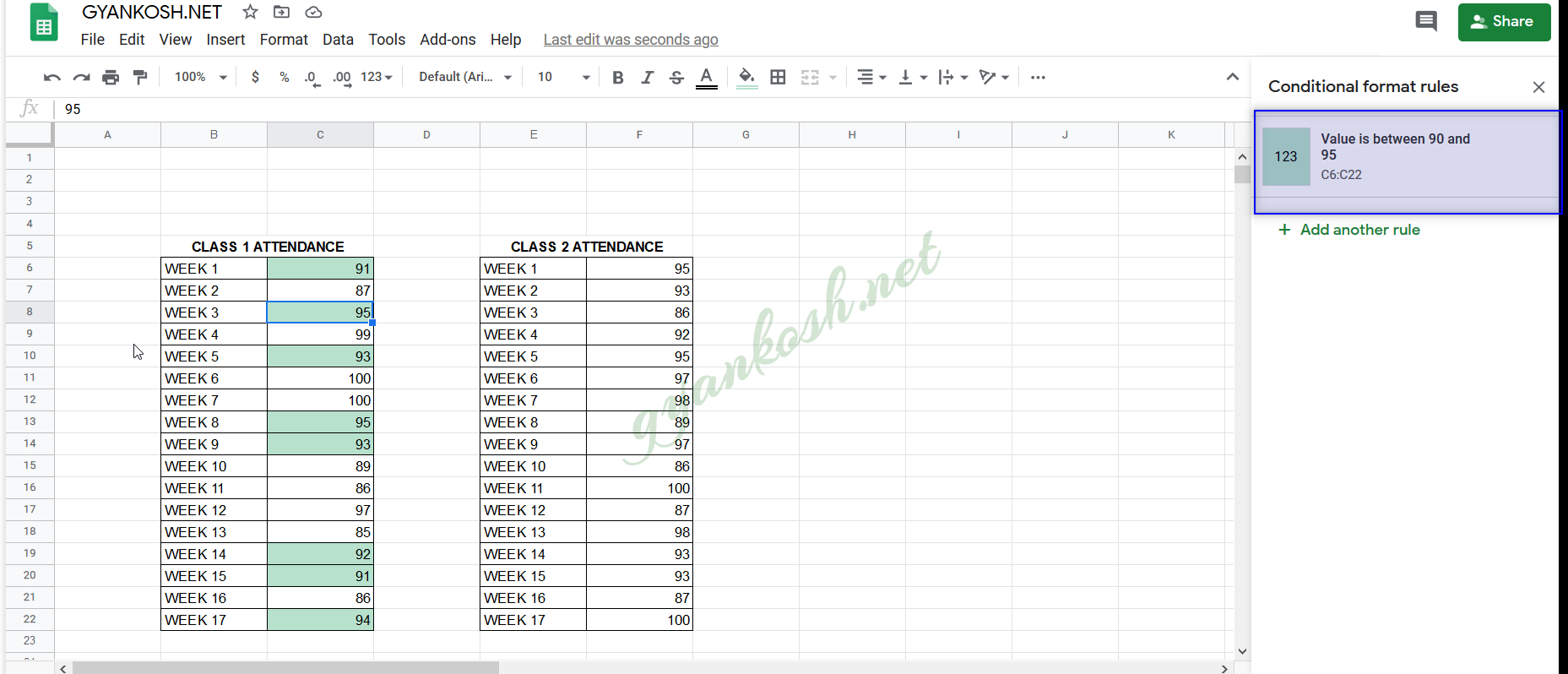
• Click the RULE which we want to copy. In this example , we have a single rule which will appear in the box.
• The Rule details will open.
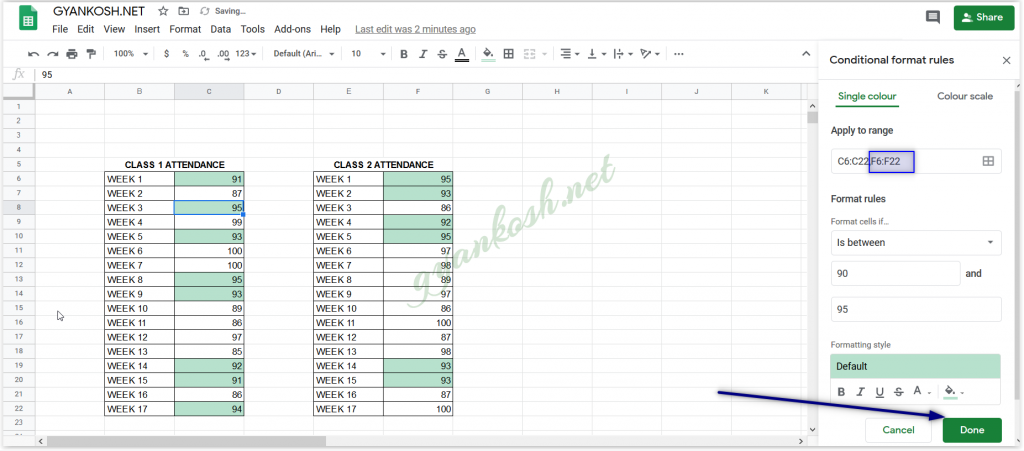
• Go to APPLY TO RANGE and add a comma [ , ] after the already present data there and write the additional range in which you want to apply the rule. FOR OUR EXAMPLE, WE WANT TO COPY THE CONDITIONAL FORMATTING ON THE CELLS F6 TO F22 SO WE ADD THIS RANGE TO THE ” APPLY TO RANGE” FIELD AS SHOWN IN THE PICTURE BELOW.
• There is no need to do anything else.
• Click DONE.
• The rule will be applied to the new table as well.
  

• Click DONE.
• The rule will be applied to the new table as well.
  
  

THE FINAL TABLE IS SHOWN IN THE PICTURE BELOW.

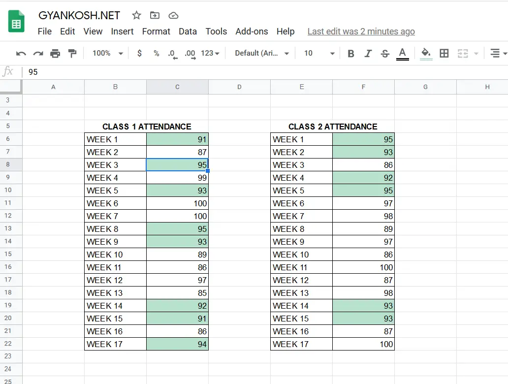
In this article we learnt the way to copy the conditional formatting [ rules ] directly so that we can save the time in repeating the procedure.

If you have any doubts, suggestions, feel free to comment.

It’ll help us make the article better.

FAQs

HOW TO COPY CONDITIONAL FORMATTING FROM ONE SHEET TO ANOTHER ?

The requirement of copying and pasting the conditional formatting across different sheets can emerge frequently. Let us try to find out the solution of this problem.

The first of the discussed solutions can be applied to copy the conditional formatting from one sheet to another.

1. The direct copy and paste conditional formatting method can be used by simply pasting the conditional formatting of one data over the other data which is present in the other sheet.

EXAMPLE DATA: We simply have a group of numbers in which we have highlighted the numbers with green color which are greater than 50.

1. FOLLOW THE STEPS
2. Click on any of the cell containing the conditional formatting rules of the table.
3. Press CTRL+C or Right Click> Copy.
4. Go to another sheet by clicking on the sheet name at the bottom.
5. Select the complete table on which conditional formatting rules is to be applied.
6. Choose RIGHT CLICK> PASTE SPECIAL> CONDITIONAL FORMATTING ONLY.
7. The conditional formatting will be copied.
8. The elaborate process with the pictures is shown above.
9. The following animation shows the process.

FAQs

CONDITIONAL FORMATTING ONLY COPIES THE CONDITIONS OR DATA TOO?

CONDITIONAL FORMATTING has nothing to do with the data but only the rules for the formatting which are applied on the particular cells.

It’ll simply copies the CELL RULES to the other cells.

WHAT IS CONDITIONAL FORMATTING ?

Conditional formatting is formatting of the selected cells on the basis of the values present in the cells. For example, if we want to highlight all the cells containing 5, we can do so.

Visit HOW TO USE CONDITIONAL FORMATTING IN GOOGLE SHEETS? for more details.

HOW TO HIGHLIGHT THE CURRENT DAY IN GOOGLE SHEETS USING CONDITIONAL FORMATTING ?

Yes , it can be done by putting a formula to compare the current day with the given data.

For the formula, you can visit

Visit HOW TO HIGHLIGHT THE CURRENT DAY OF THE WEEK USING CONDITIONAL FORMATTING IN EXCEL?

[ Although the article is meant for Excel, the formula is going to be the same for Google Sheets. ]

SUGGESTED READS:

You can visit the following articles for further learning. All these articles will make use of conditional formatting in different ways.

• HOW TO USE CONDITIONAL FORMATTING IN GOOGLE SHEETS?
• HOW TO USE CONDITIONAL FORMATTING BASED ON TEXT IN GOOGLE SHEETS?
• HOW TO USE CONDITIONAL FORMATTING BASED ON ANOTHER CELL [DROP DOWN LIST] IN GOOGLE SHEETS ?
• HOW TO CREATE A GANTT CHART IN GOOGLE SHEETS – WITH TEMPLATE
• HOW TO HIGHLIGHT THE DUPLICATE ENTRIES IN GOOGLE SHEETS