INTRODUCTION
DATES and TIME , if you are new to Excel and you have already tried using those format, I am pretty sure that you must have felt panicky at some sort of time.
It is quite obvious because when we don’t know the exact working of any system or process, we try to use it just by hit and trial method. It works sometimes and sometimes not.Here we are talking about Dates and Time in Excel. These are the tricky formats which we need frequently in our reports or charts.
Many times, we need to do operations on them. We need to put them in the conditions to trigger some event which makes it very important for us to learn the exact procedures to perform a task concerned with the dates and time.
In this article we would learn different tricks and methods to handle and manipulate Dates and Time formats so that they don’t mess up with our reports.
In this article we would learn aboutThe different ways to use DATE AND TIME to solve our day to day problems.
BEFORE READING THIS ARTICLE , IT IS REQUESTED TO VISIT THE PART I WHICH DISCUSSES THE CONCEPT OF THE DATE AND TIME IN EXCEL FOR BETTER UNDERSTANDING.
HOW TO GET THE DATE SERIAL NUMBER OF ANY DATE IN EXCEL
This might be the need for some specific case when we need to know the serial number of the Date in Excel. This can be accomplished in two ways.
1. USING THE FORMAT OPTION:
STEPS TO FIND OUT THE SERIAL NUMBER OF DATE BY FORMATTING CELLS
- Insert the date in any cell.
- As soon as the date is inserted the Excel would convert the format of the cells to DATE or CUSTOM [ For some formats which comes under custom’
- Go to HOME TAB and change the format under the NUMBER SECTION by choosing GENERAL.
- The cell would contain the serial number of the date.
2. USING THE FUNCTION
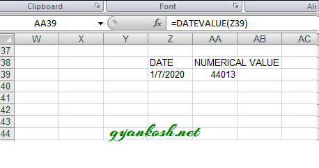
STEPS TO FIND OUT THE SERIAL NUMBER OF DATE BY USING DATEVALUE FUNCTION.
- Use the following function in the cell where serial number is needed.
- =DATEVALUE(“DATE”). It’ll return the SERIAL NUMBER of the date given.
- If the date is present in a cell, make sure the format of the cell is TEXT i.e. the DATEVALUE function would take the date as text as input.
HOW TO DISPLAY THE CURRENT MONTH AND CURRENT DAY IN WORDS IN EXCEL
While creating the reports , we might need to display any DAY [ In words] and Month [In words].
Here are the simple steps to do the same.
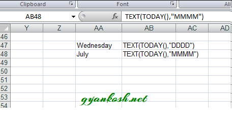
We ‘ll make use of TODAY() function which returns the current date in Excel.
Use the function in the cell as
=TEXT(TODAY(),”DDDD”)
THE FORMAT DDDD is used for Day in words.Similarly for the current month in words we’ll use the following function.
=TEXT(TODAY(),”MMMM”)
CALCULATING AGE OR NUMBER OF DAYS BETWEEN TWO DATES
Age or year,month and days between two days need to be calculated frequently in Excel. We can do that in many ways but we do have few functions to help us directly.USING DATEDIF FUNCTION
DATEDIF FUNCTION CALCULATES THE NUMBER OF DAYS , MONTH OR YEARS BETWEEN THE TWO SPECIFIED DATES.
This function calculates the age if we provide it by a starting date, an
ending date and the output type[ the form in which we need the result.
It can be years, or months or days etc.]
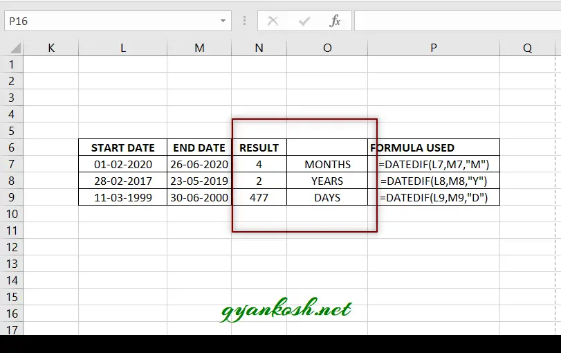
The Syntax for the DATEDIF function in Excel is
=DATEDIF(START_DATE, END_DATE, OUTPUT_OPTION)
START_DATE is the starting date from which the counting would start or the starting date of the period. This argument needs to be given in “” or as a date number. It can also be a result of any function resulting in Date.
END_DATE is the ending date till which the counting would be done or the end date of the period. This argument should also be given in “” or as a date number.
OUTPUT_OPTION is the unit in which the result is required. Refer the following table.
Use the option as per the result required.
The type of information that you want returned, where:
OPTION
“Y“
The number of complete years in the period.
“M“
The number of complete months in the period.
“D“
The number of days in the period.
“MD“
The difference between the days in start_date and end_date. The months and years of the dates are ignored.
This option is known to have issues which will be discussed later.
“YM“
The difference between the months in start_date and end_date. The days and years of the dates are ignored
“YD“
The difference between the days of start_date and end_date. The years of the dates are ignored.
COMPLETE INFORMATION OF DATEDIF FUNCTION CAN BE FOUND HERE.
Use DATEDIF FUNCTION with m , y or d option to find out the age in months , years or days simply by putting in the example.
FINDING THE EXACT AGE IN YEARS, MONTHS AND DAYS IN EXCEL
Let us find out the exact age of any person in Excel.
Say, the date of birth of a person is 21-06-2000
Find his exact age today i.e. on 2-07-2020
STEPS TO FIND OUT THE EXACT AGE
- Put the age of the person in any cell.
- Current date will be taken from the function TODAY().
- Enter the following formula in the cell where the age is needed.
- =”THE EXACT AGE OF DAVID ON ” &TEXT(TODAY(),”DD/MM/YY”)&” IS ” &DATEDIF(C17,TODAY(),”Y”)&” YEARS, “&DATEDIF(C17,TODAY(),”YM”)&” MONTHS AND , “&DATEDIF(C17,TODAY(),”MD”)&” DAYS”
FIND THE NUMBER OF DAYS BETWEEN TWO DATES
If this is the only requirement , i.e. if you want to find out the number of days between the two dates, we can always use the simple difference between the dates.
As we know that DATE is actually a number by itself. If we simply subtract the earlier date from the later one, it’ll provide us the number of days.
Suppose we have a date in cell H5 as 02-07-2020 and the other date is I5 as 30-05-2019.
We will find the number of days between H5 and I5 in J5 by putting the formula as
=H5-I5
But this function will create error if we try to subtract the date which comes late from the other one.
IF WE JUST NEED THE DIFFERENCE IN DAYS IRRESPECTIVE OF THE START DATE OR END DATE
ABS(START DATE-END DATE) OR ABS(END DATE-START DATE)
ABS function doesn’t mind with the negative values and makes everything positive. It is the same function as ABSOLUTE in mathematics.
USE THE FUNCTION AS
=ABS(H5-I5). The answer will be 399
or
=ABS(I5-H5). The answer will be 399
No errors.
WHENEVER WE FIND THE DIFFERENCE IN DAYS , WE SHOULD ALWAYS TAKE CARE OF THE DAYS TO BE CONSIDERED. SOMETHING LIKE, IF DAY 1 IS SUBTRACTED FROM DAY 2, THE MATHEMATICAL RESULT WILL BE 1 BUT IF WE WANT TO CONSIDER BOTH THE DAYS WORKING, WE NEED TO ADD 1 I.E. DIFFERENCE+1. SO ALWAYS BE CAREFUL ABOUT THIS.
FINDING OUT THE STARTING AND ENDING DATE OF THE CURRENT WEEK
This solution is for the situation when we need to find out the starting and the ending date of the week.It can be the requirement that we need to put the data in a date slab.For example it is 2nd July 2020 today.
We need to enter the data for the day under the week 28-6-2020 to 4-6-2020 which is a complete week.
Let us try to find it out automatically.The current date is given by TODAY().and there is a function called WEEKDAY() which returns the DAY number of the week i.e. 1 for the Sunday and 7 for Saturday.
WEEKDAY function takes the argument as
=WEEKDAY(serial_number,[return_type])The first argument goes through the serial number and second is the return type. The return type decided the way the days are counted for example if Sunday is 1 or Monday is 1 and so on.
GET COMPLETE INFORMATION ABOUT THE WEEKDAY FUNCTION HERE.
For the example , we will take the standard working week i.e. from MONDAY TO FRIDAY with SATURDAY and SUNDAY OFF.
STEPS TO FIND OUT THE STANDARD WEEK START DATE AND WEEKEND DATE OF THE CURRENT WEEK
- Enter the date.
- For the WEEK STARTING DATE [Week starts on SUNDAY] enter the following function
- =TODAY()-WEEKDAY(TODAY())+1
- For the WEEK ENDING DATE [Week ends on SATURDAY] enter the following function.
- =TODAY()+(7-WEEKDAY(TODAY()))
If you study the formulas, these are simple manipulations but they would work for us flawlessly. LET US GENERALIZE THE FORMULA FOR ANY DATE AND FINDING OUT THE WEEKSTART DATE AND WEEKEND DATE.We’ll just put the date in place of TODAY() in the above mentioned formulas. STEPS TO FIND OUT THE STANDARD WEEK START DATE AND WEEKEND DATE OF THE GIVEN DATE
- Enter the date. [For our example date is put in T19.]
- For the WEEK STARTING DATE [Week starts on SUNDAY] enter the following function
- =T19-WEEKDAY(T19)+1
- For the WEEK ENDING DATE [Week ends on SATURDAY] enter the following function.
- =T19+(7-WEEKDAY(T19))
ADD TIME IN EXCEL
Adding the time is again a very important utility in excel but if we don’t know the proper way to handle it, it can create problem for us.
Let us try to find out the different ways to find out the sum of time in Excel.
WHENEVER WE TRY TO PERFORM OPERATIONS ON DATE OR TIME, ALWAYS REMEMBER THAT THEY ARE NUMBERS AND TRY TO PERFORM CALCULATIONS ON NUMBERS FIRST.
We can simply add the hours as they are the number for example5:00 hrs+ 6 hrs=11 hrs.But some cases create confusion.Let us discuss the different cases one by one.STEPS TO ADD THE TIME IN EXCEL
- Enter the given times in different cells. For the example we take the two cell and put different cases in them.
- Enter the following formula in the third cell.
- =Cell 1 containing time+ Cell 2 containing time +…. so on.
- The result will appear in the result cell.[ Where we have put the formula].
EXAMPLE 1: TIME 1=5 HRS TIME 2=4 HRS.
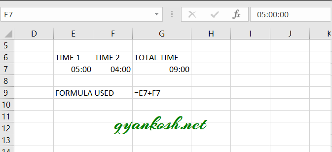
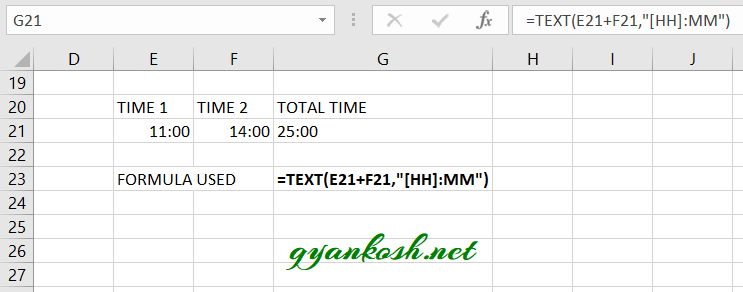
In the above picture we can see that the simple total has been performed and that is fine.EXAMPLE 2:TIME 1=11:00 HRSTIME 2=14:00 HRSLet us try to sum them up.
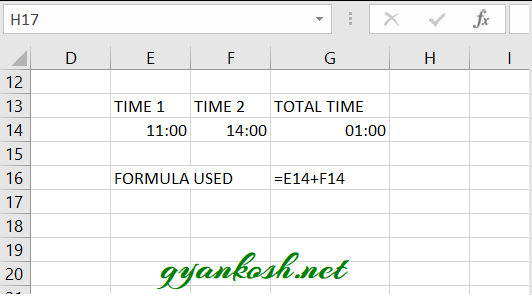
Look at the picture above.
We tried to sum 11 hrs and 14 hrs but the answer is 1 hr instead of 25 hrs.
So is it wrong??
The answer is No!!!
It is not wrong.
We know the fact that Excel sums up the hours up to 24 hours and converts it into one day.
So as soon as the sum exceeds the 24 hrs it counts it as one day and one hr.If we convert the cell to the LONG DATE [ which will show both date and time], we would find that 1:00 hr is of the next date.
But yes! we have the solution.
We’ll change the format so that we get the solution as pure hours and not dates.Revising the same example Just in place of Summing up the times, we will put it in the TEXT FUNCTION.
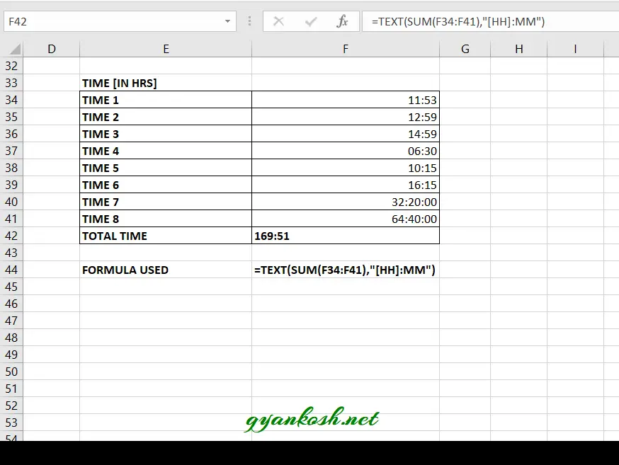
EXAMPLE 3: Let us put all the complications in this example and try our formula if it still works or not.
| TIME 1 | 11:53 |
| TIME 2 | 12:59 |
| TIME 3 | 14:59 |
| TIME 4 | 06:30 |
| TIME 5 | 10:15 |
| TIME 6 | 16:15 |
| TIME 7 | 32:20:00 |
| TIME 8 | 64:40:00 |
We use the following function for this.
=TEXT(SUM(F34:F41),”[HH]:MM”)
Where F34 to F41 has all the time stored which is summed up.
When it is summed up, it’ll change the date after every 24 hrs but as we want the result in hours only we use the TEXT FORMULA and give the format as [HH]:MM which will give the total hours and minutes as answer.
SUBTRACT TIME IN EXCEL
Let us try to learn about how to subtract time in Excel.When we are creating any worksheet regarding the time, addition and subtraction are the common operations which have to come in our way. So, it is very important to be very clear about how the time work when it is subtracted.In this section, let us try to learn how we can subtract the time in excel.
Time is just another number for Excel. We can subtract it the same way as numbers but with a bit care.
Just like the addition, we can simply subtract the time arithmetically. For example
If a cell contains 12:00 and one contains 4:00 we can simply subtract the 12:00-4:00 and the result would come as 8:00
The formula used is D8-E8.
Let us try the different cases and learn how to tackle different situations.
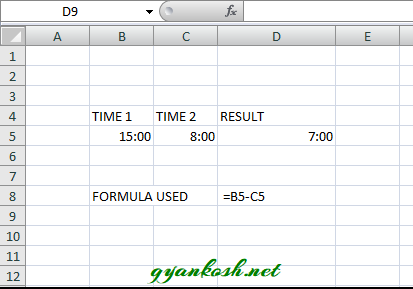
EXAMPLE 1: SIMPLE DIFFERENCE BETWEEN TIMES.
TIME 1: 15:00 HRS
TIME 2: 8:00 HRS
DIFFERENCE= TIME 1- TIME 2= 7:00
As shown in the picture below.
EXAMPLE 2: SUBTRACTING THE TIME DURING NIGHT HOURS
This particular case is for certain situations where we are calculating the work hours for a night shift.
Mostly, the night shift starts on the day 1 and ends in the morning of day 2.
This is the situation where our simple subtraction fails.
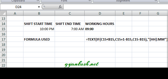
Let us try an example where the night shift starts at 10 pm and ends at 7 am.
Let us try to find out the work hours.
We put the formula as SHIFT END TIME-SHIFT START TIME [C15-B15 FOR OUR EXAMPLE] but the result didn’t show and #### appeared.
It appears when the result is negative.
WHEN WE DOESN’T MENTION THE DATE WITH A TIME, THE DEFAULT DATE IS TAKEN WHICH IS JAN 1 , 1900. ThE TIME DOESN’T GO WITHOUT A DATE WHETHER YOU MENTION IT OR NOT.
Let us try to sort this problem out.
STEPS TO FIND OUT THE TIME DIFFERENCE INCLUDING NIGHT HOURS [NIGHT SHIFT CASE]
- Put the TIME 1 as SHIFT START TIME, which is 10:00 PM in our example.
- Put the TIME 2 as SHIFT END TIME , which is 7:00 AM in our example.
- In the Working hours put the formula as
- =TEXT(IF(C15<B15,C15+1-B15,C15-B15),”[HH]:MM”)
- The formula adds a day to the morning time to make it the time of the next day so that we can perform our calculations.
- Text function is used to make the format to count hours only.
- If we need to calculate the time including many days, we need to enter dates too with the time.
- We can simply subtract the time if dates are incorporated.
HOW TO CONVERT THE TIME TO DECIMAL
While performing the calculations what if we need the decimal equivalent of any time. Yes, it is quite easy.Let us find out a few ways to get the decimal equivalent of any time.
We will discuss two ways to calculate the decimal part.
1. USING FORMAT CELLS
2. MANUAL WAY TO FIND OUT THE DECIMAL EQUIVALENT TO TIME.
1.USING FORMAT CELLS
- Place the cursor in any cell and enter the time in any of the format acceptable to Excel.
- Check if the format of the cell in the home page changed to CUSTOM or TIME. If not changed, it means Excel doesn’t recognize the format you entered.
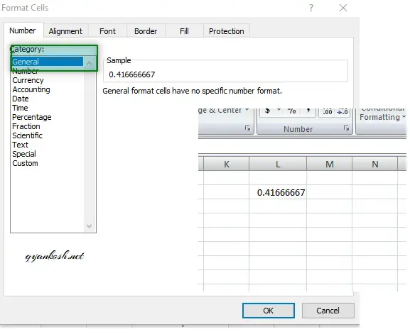
- RIGHT CLICK the cell and go to FORMAT CELLS and choose GENERAL NUMBER TYPE and click OK.
- Or go to HOME TAB and choose GENERAL NUMBER TYPE.
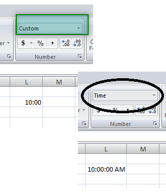
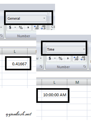
- The value in the cell will convert to the decimal number which the decimal equivalent of the time which we entered.
- Look at the picture below.
- We can see that the cell value is converted into decimal number which is the equivalent for 10 am as per our example.
2. MANUALLY FINDING THE DECIMAL EQUIVALENT OF TIME.
It is always easy if we know the concept behind any logic.
Let us try to find out the decimal equivalent of the time in excel without opening the excel.
We had already introduced the concept in our first article MANIPULATING DATE AND TIME PART -I about the same. Let us revisit this.
The time is calculated as the nth part of the complete 24 hrs.
We have 24x24x60 seconds in a day.
So our smallest unit which is a second equals to 1/86400=0.00001157and one minute is equal to =1/(24×60)=0.0006944One hour is equal to =1/24=0.041666….=0.041667
Follow the steps to find out the decimal equivalent manually.
- Open CALCULATOR in windows or manual calculator.
- Find out the total hours, minutes and seconds from the 12 AM midnight.
- Our example is 10 AM which means 10 hours 00 minutes and 00 seconds from the midnight.
- Multiply the hours with the hour factor [derived above 0.041667], minutes with the minute factor [0.0006944] and seconds with the seconds factor [0.00001157].
- The result comes out to be 10*0.041667 =0.41667.
- Let us enter it into the cell and change the format to time and check the result.
CALCULATE CURRENT TIME IN EXCEL
The current time calculation is quite easy in Excel as we already have the functions which provide us the current time.
We can make use of Now() function which gives the current date and time altogether and Today() function which gives the current date only.
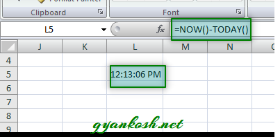
Now as we know that we need the current time only, we can subtract Today() from Now(), the integral part would be subtracted and we would be left with the decimal part only which is the time.
STEPS TO INSERT CURRENT TIME IN EXCEL
- Place the cursor in the cell where you want to insert the time.
- Put the formula =NOW()-TODAY() and click ENTER.
- The result would appear.
HOW TO INSERT THE TIME FROM TEXT IN EXCEL
Just like the date, we can insert the time from the text too.
For the date we have the DATE FUNCTION and similarly for the time we have a TIME FUNCTION.
SYNTAX for the TIME FUNCTION isTIME( HOUR, MINUTE, SECONDS).
The arguments are self explanatory.
The values go as numerals.[ numbers].If the format is General, it’ll be converted into Time.
TIME FUNCTION BECOME VERY IMPORTANT WHEN WE HAVE TO TREAT HOUR, MINUTE OR SECONDS INDIVIDUALLY AND THEN PASS THEM AS A TIME VALUE.
- The TIME FUNCTION works in such a way that it adjusts the wrong values itself. For example if you put 61 minutes, it’ll increase an hour and make the 61 minutes as 1 minutes.
- Let us try few examples to see how we can use TIME FUNCTION.
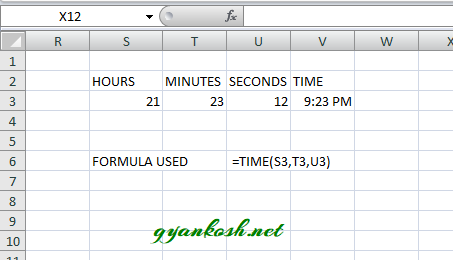
EXAMPLE 1: CONVERT THE HOURS, MINUTES AND SECONDS INTO TIME
Suppose we have been given the hours, minutes and seconds as text. Even if we try changing the format, it won’t convert it to time but we can do it using the TIME FUNCTION.STEPS TO CONVERT HOURS, MINUTES AND SECONDS INTO TIME.
- Select the cell where the output is needed.
- Enter the formula =TIME(cell containing hours value/hours, cell containing minutes value/minutes, cell containing seconds value/seconds). For our example, we have three cells containing 21, 23 and 12 as hours, minutes and seconds. So the formula used is =TIME(S3,T3,U3)
- The result will appear. Our example gave the result as 9:23 PM. We can change the format and it’ll show seconds too or we can use TEXT function for setting the format.
EXAMPLE 2: CREATING TIME FROM TEXT.
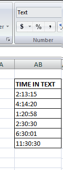
This is a specific case when we have copied any data from other source and it behaves as TEXT.
Many times we import or copy the data from other sources and all the imported data behaves as Text. It means that we won’t be able to apply any kind of calculations on that particular data as TEXT won’t respond to any calculations.
Let us take an example to understand the same.
We have the following scenario. We copied a list of dates from somewhere which are in the text format.
PLANNING FOR THE SOLUTION:
Now, if we try to sort this problem out by changing the format, it is not going to work.
But we can make use of TIME FUNCTION and separate the hour, minute and seconds parts using the LEFT, RIGHT , MID functions and pass the arguments to TIME FUNCTION. It will work as the data will be converted to time.
STEPS TO CONVERT THE TEXT INTO TIME:
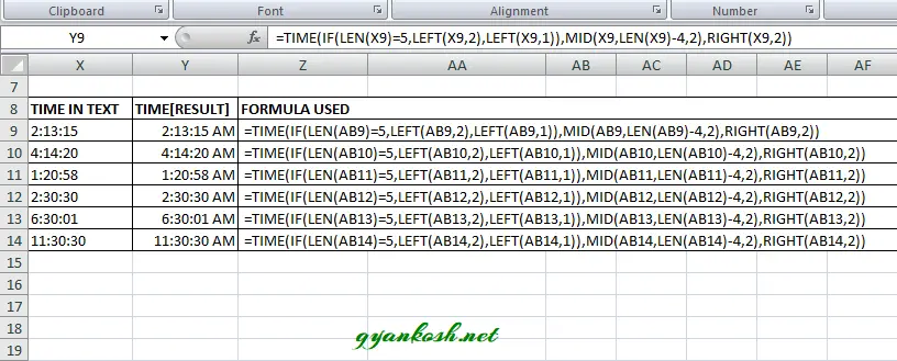
- The table is already shown and the first entry is in the cell AB9. We will create a formula for this and then drag down the formula.
- Place the cursor in the cell where we want the result .
- Enter the following formula.
- =TIME(IF(LEN(AB9)=5,LEFT(AB9,2),LEFT(AB9,1)),MID(AB9,LEN(AB9)-4,2),RIGHT(AB9,2))
- The formula would create the Time from the given time in text.
- Drag down the formula to fill all the rows of the output column.
EXPLANATION:
We are simply taking out the text snippets and passing it to the TIME FUNCTION.
Let us try to understand the formula.
=TIME(IF(LEN(AB9)=5,LEFT(AB9,2),LEFT(AB9,1)),MID(AB9,LEN(AB9)-4,2),RIGHT(AB9,2))
The formula explanation from the left.
The outer function is the TIME FUNCTION which takes the three inputs as HOUR, MINUTE and SECONDS.
We extract the HOUR from the LEFT FUNCTION. Now we can check our data that we need to decide whether we ‘ll take the one digit or two. For this case we put the IF condition which will act as per the total number of LENGTH of the string.
The second input is the MINUTES, which we extract with the help of MID FUNCTION. The MID FUNCTION starts from the length -4. The number of characters to the right are fixed but from the left it is not fixed due to the number of digits in the HOUR FIELD. So we extract it from the right and subtract the fixed position which is 4 and extract 2 letters.
The third and final extraction is easier so we use the RIGHT FUNCTION and get the last two letters.
The output is correct. The text time are converted into TIME VALUES WITH CORRECT FORMAT.
THE SAME PROBLEM CAN BE SOLVED USING THE TEXT FUNCTION TOO. BUT THE ABOVE METHOD IS MENTIONED INTENTIONALLY AS IT GIVES US MUCH MORE FLEXIBILITY AND COVERS OTHER SOLUTIONS TOO.
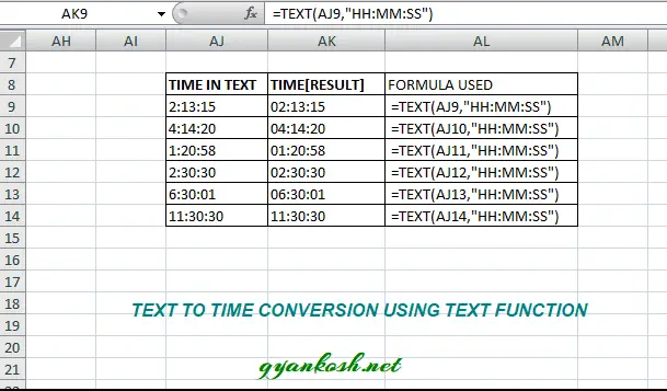
CONVERTING THE TEXT TO TIME USING TEXT FUNCTION:
We can solve this problem using TEXT FUNCTION too.
STEPS TO CONVERT TEXT TO TIME USING TEXT FUNCTION.
- Select the cell where output is needed.
- Use the function =TEXT(VALUE, “HH:MM:SS”)
- The output will be in TIME format.
CALCULATE TIME AFTER CERTAIN HOURS , MINUTES OR SECONDS IN EXCEL
A situation can arise where we need to add some time[in hours, minutes or seconds] directly to the given time.
We can add this time by making use of the TIME FUNCTION.
For Example
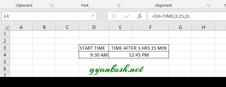
Suppose we have time in cell D4 and we need to find out the time after 3 hrs 15 minutes.
Follow the steps to find the time after certain hours, minutes and seconds.
- Select the cell where you want the result.
- Enter the formula =D4+TIME(3,15,0) and click Enter.
- The result will appear as 12:45 PM for our example which is correct.
EXPLANATION: We simply add the time using the TIME FUNCTION to the time present in a cell. TIME(3,15,0) means 3 hrs, 15 minutes and 0 seconds and they are being added to time present in the address D4.
PUTTING THE TIME IN SLOTS[ROUNDING THE TIME]
Many times the time is divided into slots and we need to take the working time from the slot only and not before that.
In such case we need to round the time to the nearest slot.
Suppose we have a situation in which the time would be taken from the next 15 min slot for example if the activity starts at 10:10 the effective time would be from 10:15.
The effective timings will be every 15 min, e.g. 10, 10:15, 10:30, 10:45 and so on.
STEPS TO CONVERT THE TIME INTO SLOTS.
- Select the cell where the slot time is to be decided.
- Put the formula as =TIME(HOUR(CELL CONTAINING THE TIME),CEILING.MATH(MINUTE(CELL CONTAINING THE TIME),15,0),0)
- For our example, the time is kept in E17 so the formula is =TIME(HOUR(E17),CEILING.MATH(MINUTE(E17),15,0),0).
EXPLANATION OF THE FORMULA USED:
=TIME(HOUR(E17),CEILING.MATH(MINUTE(E17),15,0),0)
We started with the outer function TIME, which would take three inputs as HOUR, MINUTES and SECONDS.
HOURS are extracted simply using the HOUR FUNCTION which will give the number of hours from the given time.
As we need to round off the minutes, we use the function CEILING.MATH in which we put the inputs and have given the significance of 15 minutes, seconds are zero.
Now any time would be rounded to the next 15 min slot.
MILITARY TIME IN EXCEL
MILITARY TIME is expressed as the 24 hour time but without the colon [:].
For example 1 AM as 0100 and 10:30 pm AS 2230. So the time ranges from 0000 to 2359. Let us find out the conversion of NORMAL TIME to MILITARY TIME and MILITARY TIME to NORMAL TIME.
CONVERT STANDARD TIME TO MILITARY TIME:
We can convert it simply using the TEXT FUNCTION.
STEPS TO CONVERT STANDARD TIME TO MILITARY TIME.
- Enter the standard time in a cell.
- Select the cell where we want to calculate the military time.
- Enter the formula as =TEXT(E15,”HHMM”)
CONVERT MILITARY TIME TO STANDARD TIME
We have the following challenges before we convert the military time to standard time in Excel
- The military time is not recognized by EXCEL and it is just a text.
- We need to put the military text in the time format and convert the text into time.
- We can change the format using the left and right function and can convert it to time using time value function.
STEPS TO CONVERT MILITARY TIME TO STANDARD TIME.
- Enter the MILITARY time in a cell.
- Select the cell where we want to calculate the STANDARD TIME.
- Enter the formula as =TIMEVALUE(LEFT(TEXT(E21,”0000″),2)&”:”&RIGHT(TEXT(E21,”0000″),2))
- Convert the format to time using the RIGHT CLICK>FORMAT CELLS>TIME FORMAT or GO TO HOME TAB>TIME FORMAT under NUMBER SECTION.
EXPLANATION OF THE FORMULA: CONVERSION OF MILITARY TIME TO STANDARD TIME
The formula used is =TIMEVALUE(LEFT(TEXT(E21,”0000″),2)&”:”&RIGHT(TEXT(E21,”0000″),2))
The outer function is the TIMEVALUE and it takes the text as time.
We pick the left two digits with the help of LEFT FUNCTION and right two digits with the RIGHT FUNCTION.
We used TEXT FUNCTION to make the time forcibly contain the 4 digits as if the time is before 10 am it will be shown as 3 digits in Excel for example 630,800 etc.
ONE SHORTCUT METHOD TO CONVERT MILITARY TIME TO STANDARD TIME
We can directly convert the military time to standard time by using the TEXT FUNCTION as
=TIMEVALUE(TEXT(CELL CONTAINING THE MILITARY TIME,”00\:00″))
It’ll give us the output as Timevalue which can be converted into standard time format using the format change.