Table of Contents
- INTRODUCTION
- WHEN WE NEED TO USE CONDITIONAL FORMATTING BASED ON OTHER CELL
- EXAMPLE 1:HIGHLIGHT THE NUMBERS DIVISIBLE BY THE GIVEN DIVISOR COMPLETELY
INTRODUCTION
Conditional formatting is the formatting [ font, color, fill color , size etc. ] of data as per its value of the content of the cells.
CONDITIONAL FORMATTING IS HIGHLIGHTING THE CELLS WHICH SATISFY THE GIVEN CONDITION
It is one of the most versatile functions present in Excel and very easy to apply and learn.
It makes our task so easy which you can understand from the following example.
CLICK HERE TO LEARN THE BASICS OF CONDITIONAL FORMATTING IN EXCEL
Let us lean the way to apply conditional formatting to our data.
WHEN WE NEED TO USE CONDITIONAL FORMATTING BASED ON OTHER CELL
Conditional formatting is generally done on the basis of the data or values in the cell itself but many conditions can arise when we need to given this control to the values in other cells.
WE CAN EASILY CONDITION THE CELLS TO HIGHLIGHT THE DATA ON THE BASIS OF VALUE CONTAINED IN SOME DIFFERENT CELL.
Let us try different examples and learn how we can highlight the data on the basis of another cell.
EXAMPLE 1:HIGHLIGHT THE NUMBERS DIVISIBLE BY THE GIVEN DIVISOR COMPLETELY
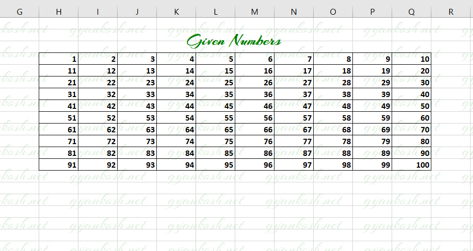
Let us take an example data of number 1 to 100.
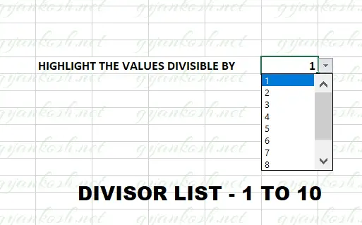
Another controlling cell will be containing the divisors from 1 to 10. [ The number that divides a number ].
The numbers which are completely divisible by the divisors should be highlighted.
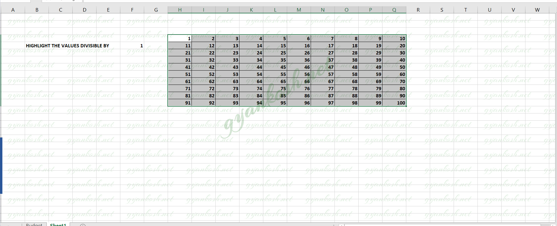
HIGHLIGHT THE NUMBERS COMPLETELY DIVISIBLE BY THE CHOSEN DIVISOR .
DATA PREPARATION
We have a data pool with number 1 to 100 as shown in the previous picture.
For the divisors, we have created a simple list containing the digits from 1 to 10 from which we ‘ll be choosing the divisor. [ CLICK HERE TO LEARN HOW TO CREATE SIMPLE DROP DOWN LIST IN EXCEL ].
CREATING CUSTOM FORMULA TO HIGHLIGHT DATA ON THE BASIS OF DIVISOR [ OTHER CELL ]
PRE-PLANNING
Let us add the custom rule to the data so that it highlight the cells containing the data which satisfy our condition.
We want to highlight the data which is the multiple of the selected number or which shows the numbers divisible by the selected divisor.
We’ll be using the function MOD [ which provides the remainder after dividing the number from the given divisor]
We’ll be using the NOT function too to flip the outcome of the MOD function.
ADD CUSTOM FORMULA TO THE DATA
FOLLOW THE STEPS TO HIGHLIGHT THE NUMBERS WHICH ARE DIVISIBLE BY THE GIVEN DIVISOR
- Select the numbers 1 to 100.
- Go to HOME TAB and choose CONDITIONAL FORMATTING DROP DOWN and click on NEW RULE.
- The NEW RULE window will open.
- Enter the new rule as =NOT(MOD(H4, $F$5)) where H4 is the first cell of the selected data and F5 is the divisor which is fixed for the reason we have given the absolute address using the $.
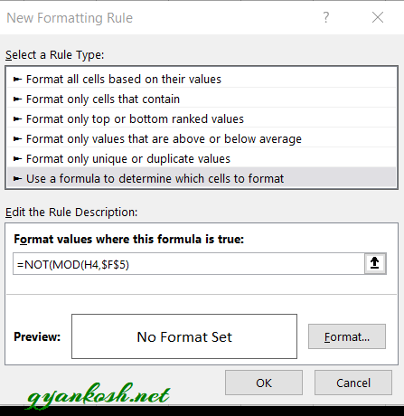
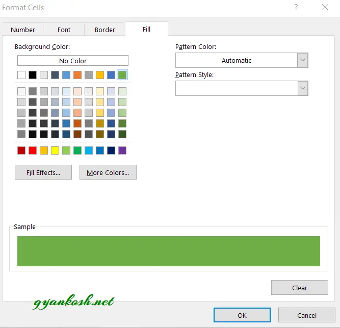
- Click on the FORMAT BUTTON so that we can choose the format of the data which will satisfy our condition.
- For our example, we have simply chosen the green fill color.
- Click OK.
- After the format is all set , Click OK.
- We’ll again reach the previous window EDIT FORMATTING RULE.
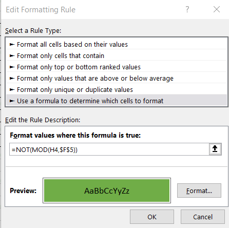
- Now, we have set the format and put the formula too, so Click OK again and we’re done setting the rule for conditional formatting .
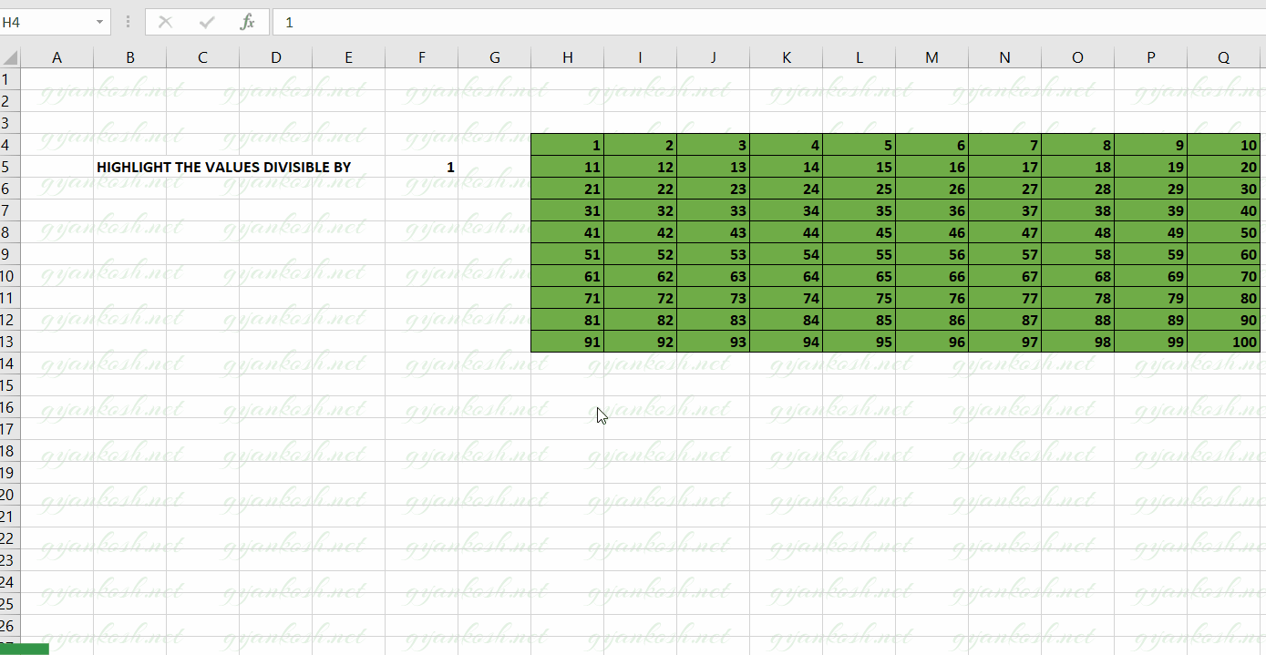
- As soon as we click OK, we’ll see that all the data is green as the divisor is selected as 1. It is clear that all the digits are divisible by 1 and no remainder is left.
- Now, let us try check our example.
- Change the divisor from the given list, and see the effect.
- The following animation shows the running of our example, which works perfectly fine.
So, in this example we saw that we changed the highlighting rules on the basis of the value which is contained in another cell, which is not a part of the data.
We’ll add more examples to the same article, keep checking.
Please share your views and give suggestions to make this article even better.