Table of Contents
- INTRODUCTION
- HOW TEXT IS HANDLED IN EXCEL?
- SPLIT CELLS IN EXCEL
INTRODUCTION
Whenever we prepare any report in excel, we have two constituents in any report.
The Text portion and the Numerical portion.
But just storing the text and numbers doesn’t make the super reports. Many times we need to automate the process in the reports to minimize the effort and improve the accuracy.
Many functions are provided by the Excel which work on Text and give us the useful output as well. But few problems are still left on which we need to apply some tricks with the available tools.
In this articles , we are going to separate or split the text into different parts.
HOW TEXT IS HANDLED IN EXCEL?
TEXT is simply the group of characters and strings of characters which convey the information about the different data and numbers in Excel. Every character is connected with a code [ANSI].
Text comprises of the individual entity character which is the smallest bit which would be found in Excel.
We can perform the operations on the strings[Text] or the characters.
Characters are not limited to A to Z or a to z but many symbols are also included in this which we would see in the later part of the article.
TEXT IS AN INACTIVE NUMBER TYPE[FORMAT] IN EXCEL.
ANYTHING STORED AS TEXT [NUMBER OR DATE] WON’T RESPOND TO ANY STANDARD FORMULAS OR FUNCTIONS BUT SPECIALLY DESIGNED TEXT FUNCTIONS. [EXCEPTIONS DO OCCUR IN CASE OF NUMBERS]
If we need to make anything inactive, such as Date to be non responding to the calculation, we put it as a text. Similarly if we want to avoid any calculations for a number it needs to be put as a text.
SPLIT CELLS IN EXCEL
SPLITTING/SEPARATING the text is also required many times in Excel.
This can be stated as removing any portion of the text or string from the cell and place it into the different cells.
Splitting and separating the cells can be done in a many ways. For example
- TEXT TO COLUMN– We can split the text in a cell into the different columns. The basis of the separation can be any delimiter like a comma, colon etc.
- USING FLASHFILL
- Separating a single word into many portions.
- Separating Text on the basis of any character or pattern
TEXT TO COLUMN:
We’ll discuss it here briefly as a complete detailed topic is already present.
CLICK HERE TO CHECK OUT THE COMPLETE ARTICLE ON TEXT TO COLUMN.
Text to column is used in a situation when we need to split any string [sentence of few words] separated by any delimiter [ comma, colon , full stop, semicolon, space etc. The process is backed up by a wizard mechanism which makes it very simple. The only requirement is that it needs a delimiter, some character on the basis of which it’ll separate the string into words.
USING FLASHFILL:
FLASH FILL is a new tool for many kind of task which would otherwise take much time. For such tricky tasks such as separating the words or auto filling or many such kind of tasks which has some pattern are well suited for the FLASH FILL. It is a complete topic discussed in detail.
CLICK HERE TO CHECK OUT THE COMPLETE ARTICLE ON FLASH FILL IN EXCEL.
SPLIT TEXT INTO MANY FRAGMENTS:
In this section we will learn to separate any text into many portions even if there is no delimiter. [Of course if we’d be having delimiter we’ll be using Text to Column option].
We perform this action with the use of LEFT, RIGHT AND MID FUNCTIONS.
LEFT FUNCTION has the capability to pick the specified number of characters from the left side of the text.
RIGHT FUNCTION can extract the specified number of characters from the right whereas
MID FUNCTION takes out the specified number of the characters from the middle of the text.
Let us find out the way we can use these functions to extract the values from the text.
EXAMPLE 1: SEPARATING THE DATE IN EXCEL
This problem occurs mostly when we have imported the data from somewhere and the date is in some format which doesn’t suit our system. The date can also be without any delimiter just like
11032011
12032011
13032011
and so on.
SOLUTION:
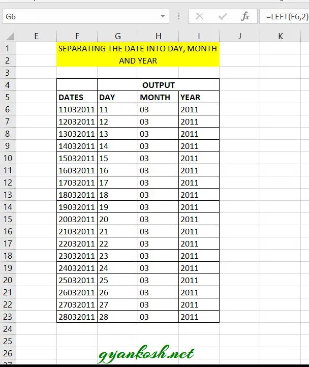
In this problem , first of all we have to check the pattern. We can see that the left two digits are the dates, after that the month and then the year.
If we want to put the date, month and year in the separate columns, put the following functions in the column for
DATE, MONTH AND YEAR.
FORMULA FOR DATE COLUMN =LEFT(CELL CONTAINING THE DATE,2) [PICKING 2 LETTERS FROM THE LEFT]
FORMULA FOR MONTH COLUMN =MID(CELL CONTAINING THE DATE,3,2) [STARTING FROM THE LETTER POSITION 3, PICKING 2 LETTERS]
FORMULA FOR YEAR COLUMN =RIGHT(CELL CONTAINING THE DATE,4) [PICKING 4 LETTERS FROM THE RIGHT]
The result will be the date, month and year separated and in three columns.
EXAMPLE 2: SPLITTING A RANDOM TEXT IN PARTS
To further understand the usage of functions LEFT, RIGHT and MID, let us take one more example and check how we can use them.
Suppose we have the WEEKDAYS LIST and we need to limit the letters upto 4 only.
We can simply use the LEFT FUNCTION.
To Extract the 4 letters from the left of the weekdays we can use the formula as =LEFT(CELL CONTAINING WEEKDAY,4). It’ll extract the letters from the left as shown in the picture below.
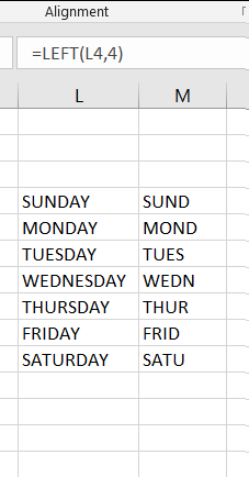
If we look at the results, we can see that the function did what we wanted but as per standards , in a week we sometimes take 4 letters and sometimes 3 letters from the left. Let us refine the function and make it proper.
We know that the 4 letters are taken for TUESDAY ONLY. We can put an IF function in a way as
=IF(L4=”TUESDAY”,LEFT(L4,4),LEFT(L4,3))
If the day is TUESDAY , 4 letters would be taken from the left otherwise only 3 will be taken from the left.
The result is shown in the picture below which is better than the previous one.
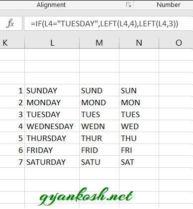
THERE ARE MANY STANDARDS OF THE SHORT FORMS OF THE WEEKDAYS. THE MOTIVE HERE IS TO UNDERSTAND THE USAGE OF THE FUNCTION.
Similarly we can split any text if we know the position of the split.
Let us find out the way to split the text if we don’t know the position exactly.
SPLITTING/SEPARATING TEXT ON THE BASIS OF PATTERN OR PRESENCE OF CHARACTER:
Let us now check out the most important part of the search and split trick in Excel.In this process we need to search for a character and then act according to the situation.We would learn this process using the examples.
SPLITTING FIRST NAME AND LAST NAME IN EXCEL:
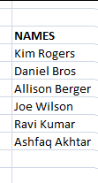
Suppose we have a column with the first and last name put in the same cell.
If we want to apply any kind of formula on this, we need to separate or split the first and last name.
Suppose the data given is
Kim Rogers
Daniel Bros
Allison Berger
Joe Wilson
Ravi Kumar
Ashfaq Akhtar
We can do that using the following methods.
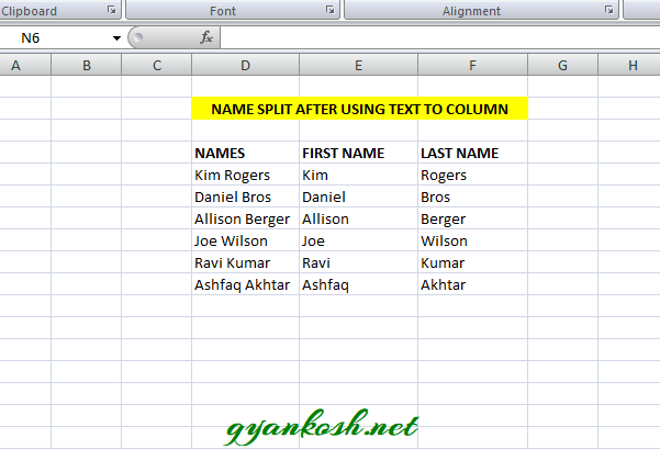
1. TEXT TO COLUMN–
We can use this trick confidently and easily to separate the first and last name within seconds. [CLICK HERE TO LEARN TEXT TO COLUMN WITH PICTURES AND EXAMPLES].
After applying the text to column, we will be having the following data.

2. USING FLASH FILL TO SPLIT NAMES OR TEXT:
As already discussed we can use FLASH FILL also to separate the names into first name and last name in Excel.
[CLICK HERE TO LEARN FLASH FILL IN EXCEL]
STEPS TO USE FLASH FILL:
Attempt one sample manually. For our example Split the first row which is Kim Rogers as Kim and Rogers in the other column as shown in the picture.
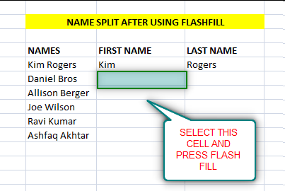
- Select Next cell to continue the process.
- Click DATA>FLASH FILL.
- If EXCEL has understood the pattern , the next name i.e. Daniel will be filled here. The complete column will be filled automatically.
- Similarly select LAST NAME for DANIEL BROS and click FLASH FILL. The complete column will be filled.
- We are done.
3. USING FUNCTIONS TO SPLIT NAMES OR ANY TEXT INTO PARTS
After the automated options let us try now the manual one, of course using the functions.
Here are our requirements.
A function which can
- Search any character [We can use SEARCH function or FIND for the same.
- Functions which can extract characters from the TEXT. [LEFT, MID AND RIGHT FUNCTION are the best contenders for this task].
- Function which can return the length of the text. [LEN FUNCTION is suitable for this task].
With the use of these function , let us try to separate the text in Excel.
EXAMPLE 1: SPLITTING THE NAMES USING FUNCTIONS IN EXCEL:
Let us try our same example first.
STEPS TO SPLIT THE NAMES WHICH CONTAIN SPACE AS THE SEPARATOR
- Select the cell where we want the first name.
- Enter the formula as =LEFT(D17,SEARCH(” “,D17,1)-1) where D17 is the cell containing the NAME. [In this step we use the LEFT function to extract the characters from the left. We take the first input as the cell containing the complete name,. The second input is taken with the help of Search function which will compare space ” ” in the complete name from the character 1 and return the position of the space, which will become the length of the characters from the left.
- Enter the formula =RIGHT(D17,LEN(D17)-SEARCH(” “,D17,1)) [This function works on the same priciple as the previous step. The function is RIGHT and takes the first argument as the complete name which is in D17 for our example. The LEN(D17) returns the complete length of the string. We subtract the location of the SPACE ” ” using the same method which is using the SEARCH FUNCTION. This combination gives us the location of the starting of the second word.
- Drag both the formulas down the column.
- The result is shown in the pic.
EXAMPLE 2: SPLITTING THE NAME/TEXT OF MORE THAN TWO WORDS IN EXCEL
We just learnt how to separate the Names in two different cells. Now let us learn to separate the names which contain a Middle name into Three different portions.
STEPS TO SPLIT THE NAMES WHICH CONTAIN MIDDLE NAME TOO.
- Select the cell where we want the first name.
- Enter the formula as =LEFT(H4,SEARCH(” “,H4,1)-1) where H4 is the cell containing the NAME. [In this step we use the LEFT function to extract the characters from the left. We take the first input as the cell containing the complete name,. The second input is taken with the help of Search function which will compare space ” ” in the complete name from the character 1 and return the position of the space, which will become the length of the characters from the left.
- For the middle name we need to use the MID FUNCTION. Select the cell for the MIDDLE NAME and put the following formula =MID(H4,SEARCH(” “,H4,1)+1,SEARCH(” “,H4,SEARCH(” “,H4,1)+1)-SEARCH(” “,H4,1)) . [The function starts with MID as the top function. The first argument is the H4 which is the cell containing the complete name. The second argument is the starting character sequence number. We used SEARCH FUNCTION and try to search ” ” in H4. We add one to this as we need the first letter of the middle name. The third argument is the number of letters to be taken for the middle name. We found it out using the SEARCH FUNCTION again but started the SEARCH FROM THE NEXT SPACE” ” which would return the space after the middle name or second word. Subtract this position from the position of the first space. Now we have the number of letter we want.
- The LAST NAME or the third word can be found by using the following formula. Enter the formula in the LAST NAME COLUMN AS =RIGHT(H4,LEN(H4)-(SEARCH(” “,H4,SEARCH(” “,H4,1)+1))) [This function works on the same priciple as the previous step. The function is RIGHT and takes the first argument as the complete name which is in D17 for our example. The LEN(D17) returns the complete length of the string. We subtract the location of the SPACE ” ” using the same method which is using the SEARCH FUNCTION. This combination gives us the location of the starting of the second word.
- Drag both the formulas down the column.
- The result is shown in the pic.