Table of Contents
- INTRODUCTION
- WHAT IS MEANT BY ROTATING A TABLE?
- ROTATING A TABLE IN EXCEL
- 1. USING RIGHT CLICK OPTION
- 2. ROTATE TABLE USING TRANSPOSE FUNCTION IN EXCEL
- STEPS TO ROTATE THE TABLE USING TRANSPOSE FUNCTION
INTRODUCTION
Suppose we have a data which needs to be rotated i.e. the rows should become the columns and vice versa. How would we do that?
One method is , to create a new sheet and start doing this manually but would that be an efficient solution. What if the report is too big like 1000 lines or so.
The article is about rotating a table i.e. Column becomes the rows and rows become the column or we can say rotate the table by 90 degrees.
This kind of need can emerge from any specific requirement or the layout issues. But whatever be the reason, we should always be ready for such a situation and that is why we are going to discuss this issue here.
We’ll discuss the different ways of rotating a table in excel.
The solution to our problem is given by a function named Transpose which is a technical term for rotating any data. We can perform this task in two ways mainly.
We’ll discuss both in details in this article.
WHAT IS MEANT BY ROTATING A TABLE?
A table is made up of rows and columns.
Rotating the data means converting rows to columns or rows to columns.
It can also be said that we change the layout of the table from portrait to landscape or landscape to portrait.
This is required when we want to fetch the data from a table already lying in a different manner than the target table.
ROTATING A TABLE IN EXCEL
We’ll discuss the different ways of rotating a table in excel.
The solution to our problem is given by a function named Transpose which is a technical term for rotating any data. We can perform this task in two ways mainly.
1. Using RIGHT CLICK SPECIAL PASTE menu.
2. Using TRANSPOSE FUNCTION
1. USING RIGHT CLICK OPTION
We can rotate the table using the RIGHT CLICK SPECIAL PASTE Menu. Before understanding the logic, let us perform the task first. Here are the steps to rotate the table using Special Paste. Suppose we have the following table.
| CLASS ID | LENGTH | BREADTH |
| 12 | 234 | 121 |
| 23 | 432 | 322 |
| 34 | 343 | 211 |
| 45 | 232 | 122 |
| 56 | 454 | 345 |
| 67 | 342 | 123 |
| 78 | 233 | 123 |
STEPS:
- Select the complete table which you want to rotate including the headers.
- Press CTRL+C or RIGHT CLICK> COPY.
- Select the cell where you want to paste the Rotated table and RIGHT CLICK. [ The first cell of the rotated table will be filled at the cell selected]
- GO TO PASTE SPECIAL.
- The following dialog box will open.
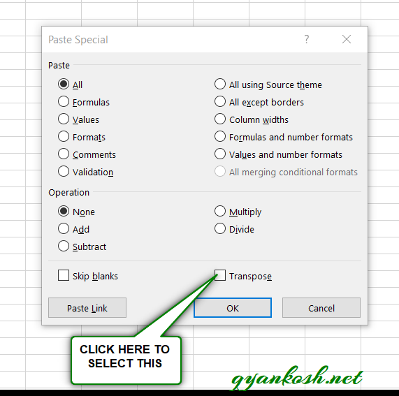
- Click on the TRANSPOSE CHECKBOX on the lower right bottom of the dialog box.
- Click OK.
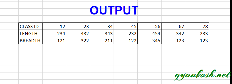
- The table will be properly pasted but the layout will be rotated.
- The output table is shown below.
2. ROTATE TABLE USING TRANSPOSE FUNCTION IN EXCEL
The table can also be rotated using a function.
This can be done with the use of a function named as TRANSPOSE FUNCTION. [ CLICK HERE FOR FULL INFORMATION]
For a review the syntax ( the way how formula is phrased for excel) of MATCH is
=TRANSPOSE(ARRAY OF CELLS)
ARRAY ARRAY IS A GROUP OF CELLS WHICH CAN BE DECLARED AS A RANGE .
ARRAY can be like A1:A10
OR
A1:C10 with three columns and ten rows
or
{1;2;3;4}
STEPS TO ROTATE THE TABLE USING TRANSPOSE FUNCTION
Here are the steps to rotate the table using transpose function.
Let us try to transpose the following table.
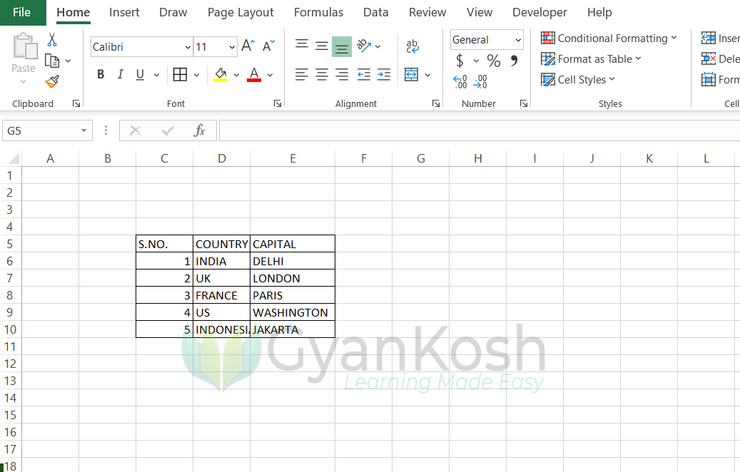
Suppose the following TABLE is present
| S.NO. | COUNTRY | CAPITAL |
| 1 | INDIA | DELHI |
| 2 | UK | LONDON |
| 3 | FRANCE | PARIS |
| 4 | US | WASHINGTON |
| 5 | INDONESIA | JAKARTA |
We will transpose this array using the TRANSPOSE function.
STEPS:
Follow the following steps to rotate the table in EXCEL.
REFER PICTURE: ABOVE
1. Check the number of rows and columns of the given table. e.g. our example table has 3 columns and 6 rows.
Now select the layout for the transposed table i.e. 3 rows and 6 columns.
Now do nothing, and start typing the formula starting with an “=”. The selection won’t be removed.
2. Now type the formula
=TRANSPOSE(C3:E8) but don’t PRESS ENTER.
3. Press CTRL+SHIFT+ENTER.
4. The selected table will be rotated. [transposed]
But if you are having OFFICE 365 or any later versions, you can follow the procedure given below.
The CSE method discussed above applies to the EXCEL VERSIONS prior to OFFICE 365.
IF YOU HAVE OFFICE 365 OR LATER, NO NEED TO USE THE CTRL+SHIFT+ENTER.
USE THE FUNCTION SIMPLY AS YOU USE THE OTHER FUNCTIONS. THE RESULT WILL BE CORRECT.
STEPS TO ROTATE THE TABLE IN OFFICE 365 OR LATER:
Follow the following steps to rotate the table in EXCEL.
REFER PICTURE: BELOW
1. We need not to care about the number of columns or rows in Office 365 or later Excel version.
Now select the layout for the transposed table i.e. 3 rows and 6 columns.
Now do nothing, and start typing the formula starting with an “=”. The selection won’t be removed.
2. Now type the formula
=TRANSPOSE(C3:E8) .
3. Press ENTER.
4. The selected table will be rotated. [transposed]