Table of Contents
- INTRODUCTION
- NUMBER OF OCCURRENCES IN A COLUMN WHEN THE DATA IS NUMBER
- NUMBER OF OCCURRENCES OF A TEXT IN A COLUMN IN EXCEL
INTRODUCTION
Knowledge is not complete unless we know how to apply it in our day-to-day applications.
So we’ll try to learn a new trick which is going to be very useful in day-to-day work
The trick to be discussed is HOW TO COUNT THE NUMBER OF OCCURRENCES IN A COLUMN, which means if there are a lot of repeated terms in a column and we need to find out the frequency of each term i.e. the number of repetitions.
I have seen many people getting puzzled about how to achieve this. In this article, we’ll check out various ways to sort this problem out.
We’ll discuss it in two parts.
1. When the data is numbers only.
2. When the data is text.
NUMBER OF OCCURRENCES IN A COLUMN WHEN THE DATA IS NUMBER
Let us first discuss the scenario when we have a complete column filled with numbers and we need to find out the occurrences of some specific values.
The sample data is given below. These are the random numbers between 11 to 20.
| 16 | ||||
| 14 | ||||
| 16 | ||||
| 14 | ||||
| 15 | ||||
| 15 | ||||
| 12 | ||||
| 17 | ||||
| 18 | ||||
| 19 | ||||
| 18 | ||||
| 20 | ||||
| 17 | ||||
| 16 | ||||
| 20 | ||||
| 14 | ||||
| 12 | ||||
| 19 | ||||
| 12 | ||||
| 16 |
We’ll sort this problem out using the following methods
1. Using FREQUENCY FUNCTION.
2. Using UNIQUE AND COUNTIF.
1. USING FREQUENCY FUNCTION
First of all, let us revise the FREQUENCY FUNCTION.
Frequency function returns the number of occurrences in given class intervals. Although it is a statistical function but we can use it here.
The syntax of the frequency function is
=FREQUENCY (DATA , BIN ARRAY)
DATA is the range or array in which we want to find out the frequency of different numbers.
BIN ARRAY is the slabs of the numbers in which we want to find out the frequencies.
*BIN ARRAY is like a limit. e.g. if we want to define three slabs like 0-10, 10-20, 20-30 , our bin array will be 10.20,30.
The complete reference is here.
CLICK HERE TO GET MORE INFORMATION ABOUT FREQUENCY FUNCTION.
PLANNING THE SOLUTION
We need two arguments to be used in the frequency function.
One is the data, which we already have.
Other is the bin array or the intervals.
Now for this, as we have random numbers and the limit we know. We’ll make the array from 11 to 20 in a column which we call as bin array column as we have the numbers from 11 to 20.
Now suppose we need to find out the number from 11-15 and 16-20, our bin array will be 15,20
But here, we want all the number’s frequencies, we’ll take all the numbers and the bin array will be 11,12,13,14,15,16,17,18,19,20 in a column.
STEPS
- In adjacent to the data , create a column of the BIN ARRAY.
- Type the numbers in the bin array. As in our case we’ll write from 11 to 20.
- Now , as, FREQUENCY FUNCTION returns the dynamic array, we need to follow the style of dynamic array declaration.[FOR OTHER THAN OFFICE 365 USERS. THEY JUST NEED TO SIMPLY USE THIS FUNCTION ]
- Select the result column upto the length of the bin array as the result will be equal to the length of bin array.
- Without deselecting start typing the formula in the first cell =FREQUENCY(DATA, BIN ARRAY) but don’t press enter.
- Press CTRL+SHIFT+ENTER shortly also known as CSE.
- The result will appear against the bin array which will show us the repetition of different numbers.
- The complete process is summarized in the animated picture below.
EXPLANATION
- The data is stored in F7 to F 26.
- The bin array is stored in G7 to G16
- The result is found in H column.
- The formula used is =FREQUENCY(F7:F26,G7:G16).
- After entering the formula we press CRTL+SHIFT+ENTER in place of a simple ENTER as explained above. Because it is an array formula. [IN OFFICE 365 WE NEED NOT USE CSE SYSTEM. SIMPLE FUNCTION INSERTION WILL WORK]
- The output is as per expectations. The data can be verified manually too.
USING UNIQUE FUNCTION
First of all let us revise the UNIQUE FUNCTION.
UNIQUE FUNCTION returns a list of UNIQUE VARIABLES from the given list
or range. It filters out the repeated data and keeps the unique data.
SYNTAX:
=UNIQUE(ARRAY to be operated, by rows/columns, Exactly once /All)
The UNIQUE function has the following arguments:
ARRAY to be operated It is the array that needs to be searched for unique values.
by rows/columns [optional, default-false] if true- Search for repeated rows if false-search for repeated columns
Exactly once/All [optional, default-false] if True, will result only those entry which occur only once. If false, will result those entries also which occur more than once [of course will return a single copy]
CLICK HERE TO GET FULL INFORMATION ABOUT UNIQUE FUNCTION.
COUNTIF:
COUNTIF FUNCTION returns the total number of cells from a given data set or range which fulfill a particular given criteria.
SYNTAX:
=COUNTIF(RANGE, CRITERIA)
RANGE Given range which needs to be scanned to find out the number of cells which fulfill the criteria
CRITERIA The criteria on the basis of which , cells will be counted.
NOTE* CRITERIA NEEDS TO BE GIVEN IN THE “”.
PLANNING THE SOLUTION
The UNIQUE FUNCTION returns the array of the unique values.
So the plan is to find out all the unique values and then finding out the count of these unique values.
UNIQUE FUNCTION needs the following inputs.
Array is the given data.
Second argument will be false as we will check the duplicate rows.
Third argument will be false as we want to count all the entries.
COUNTIF function will need two arguments.
The range and the criteria.
The range will be output of the UNIQUE FUNCTION and criteria will be that the value to be matched should be equal to the number itself so that the count of the number can be retrieved.
STEPS
- In adjacent to the data , create a column for the UNIQUE VALUES.
- Apply the unique function =UNIQUE(“RANGE”,FALSE,FALSE).
- The output will create an array of all the unique values. (UNIQUE IS AN ARRAY FUNCTION BUT WE DON’T NEED CTRL+SHIFT+ENTER HERE AS THIS IS AN OFFICE 365 FUNCTION AND OFFICE 365 USES DYNAMIC ARRAYS. IT ITSELF CREATES THE ARRAY)
- Now, in the new RESULT COLUMN put the following function to find out the occurrences of all the unique values. The formula used is =COUNTIF(OUTPUT ARRAY OF UNIQUE FUNCTION, CELL ADDRESS OF UNIQUE VALUE WHICH IS OUTPUT OF UNIQUE FUNCTION)
- Drag the function down up to the length of unique values output.
- The problem is solved.
EXPLANATION
- The data is stored in E5 to E24.
- The UNIQUE VALUES are taken as the output of the unique function in F5:F12. The function used is =FREQUENCY(E5:E24,FALSE,FALSE) as we want to find out the unique values in the given range, in column taking into consideration all the values present.
- The final result is taken in the column G with the formula used in G5 as =COUNTIF($E$5:$E$24,F5). In this formula we made the absolute references by putting a $ sign so that the lookup range doesn’t change when we drag the formula. The second value is the value for which the occurrences are to be counted. This is the value which is unique.
- Drag down the formula and result will appear for all the instances as shown in the picture.
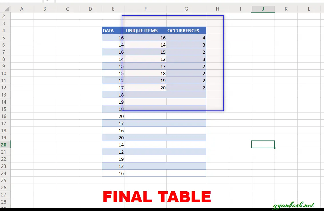
FINAL OUTCOME
Following picture shows the final outcome of the table. We achieved what we wanted.
NUMBER OF OCCURRENCES OF A TEXT IN A COLUMN IN EXCEL
Let us first discuss the scenario.
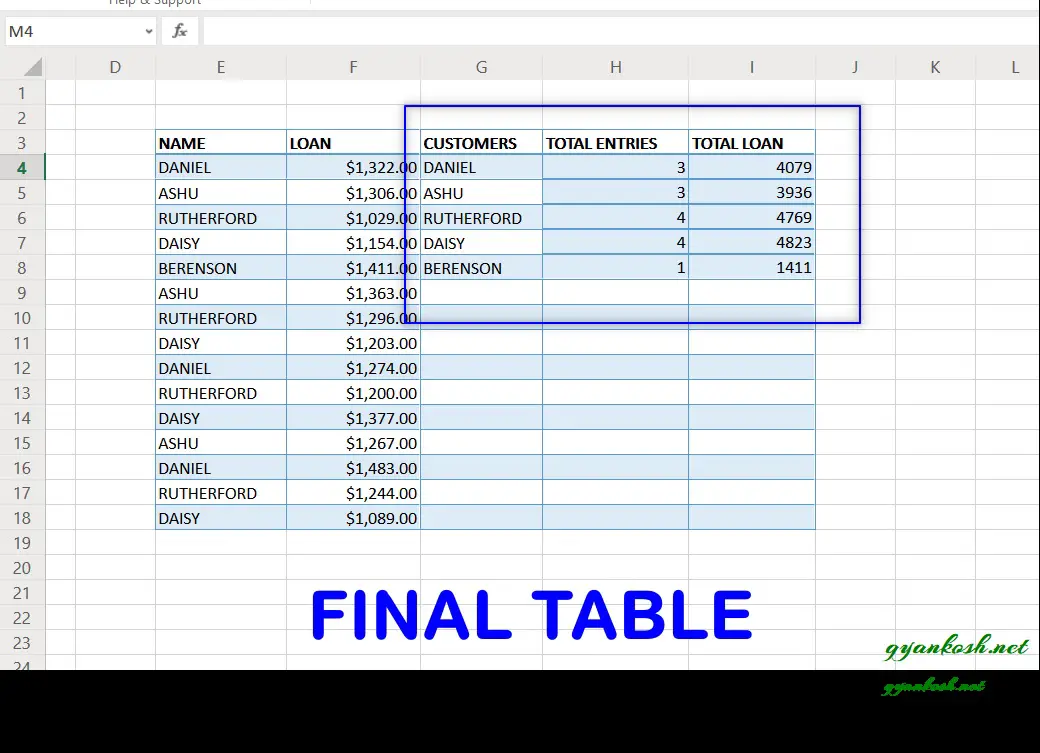
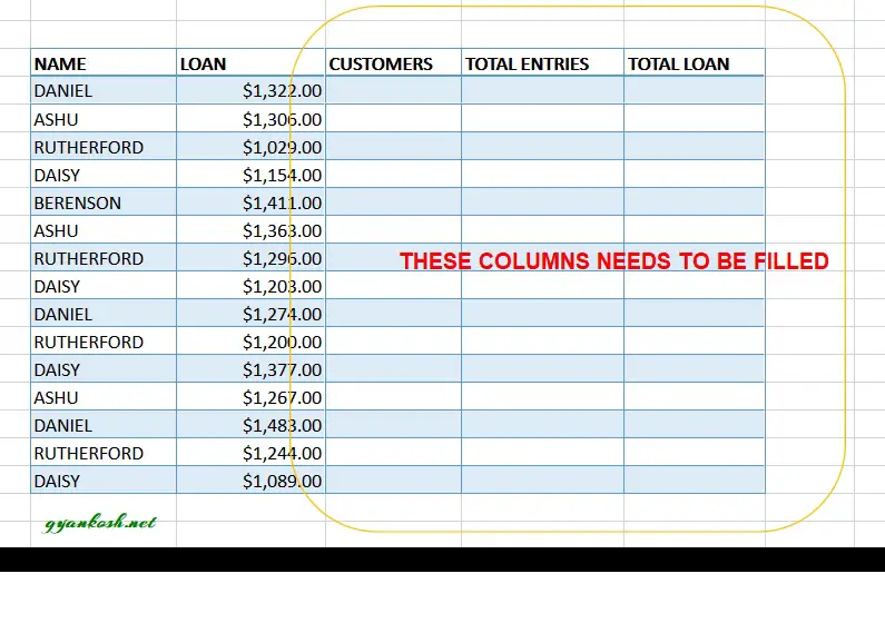
We have a loan agency and we are disbursing loans to different customers. But due to some mistake , rather than keeping a proper accounts the entries were done in a random fashion.
Now we need to find out the number of entries and total loan against every customer in the ledger.
| NAME | LOAN |
| DANIEL | $1,322.00 |
| ASHU | $1,306.00 |
| RUTHERFORD | $1,029.00 |
| DAISY | $1,154.00 |
| BERENSON | $1,411.00 |
| ASHU | $1,363.00 |
| RUTHERFORD | $1,296.00 |
| DAISY | $1,203.00 |
| DANIEL | $1,274.00 |
| RUTHERFORD | $1,200.00 |
| DAISY | $1,377.00 |
| ASHU | $1,267.00 |
| DANIEL | $1,483.00 |
| RUTHERFORD | $1,244.00 |
| DAISY | $1,089.00 |
We’ll sort this problem out using the following methods
1. Using FREQUENCY FUNCTION. IT-NOT APPLICABLE AS FREQUENCY FUNCTION WORKS FOR NUMBERS ONLY BUT WE CAN PLAY WITH DATES IF WE HAVE DATES IN THE QUESTION.
2. Using UNIQUE AND COUNTIF. -YES, IT WOULD WORK.
USING UNIQUE, SUMIF AND COUNTIF FUNCTION
First of all let us revise the the functions which are to be used so that we understand their importance in this context.
UNIQUE FUNCTION:
UNIQUE FUNCTION returns a list of UNIQUE VARIABLES from the given list
or range. It filters out the repeated data and keeps the unique data.
SYNTAX:
=UNIQUE(ARRAY to be operated , by rows/columns , Exactly once /All)
The UNIQUE function has the following arguments:
ARRAY to be operated It is the array which needs to be searched for unique values.
by rows/columns [optional, default-false] if true- Search for repeated rows if false-search for repeated columns
Exactly once/All [optional, default-false] if True, will result only those entry which occur only once. If false, will result those entries also which occur more than once [of course will return a single copy]
CLICK HERE TO GET FULL INFORMATION ABOUT UNIQUE FUNCTION.
COUNTIF:
COUNTIF FUNCTION returns the total number of cells from a given data set or range which fulfill a particular given criteria.
SYNTAX:
=COUNTIF(RANGE, CRITERIA)
RANGE Given range which needs to be scanned to find out the number of cells which fulfill the criteria
CRITERIA The criteria on the basis of which , cells will be counted.
NOTE* CRITERIA NEEDS TO BE GIVEN IN THE “”.
CLICK HERE TO GET FULL INFORMATION ABOUT COUNTIF FUNCTION.
SUMIF FUNCTION:
SUMIF function adds us the
different given values or a range only if a particular criteria is met,
otherwise it rejects the calculation.
SYNTAX:
=SUMIF(LOOKUP_RANGE, CRITERIA, SUM_RANGE)
LOOKUP_RANGE The range which will be searched for the criteria
CRITERIA criteria to be checked on
SUM_RANGE The values which will be summed up if criteria is true.CLICK HERE TO GET COMPLETE KNOWLEDGE ABOUT SUMIF FUNCTION
PLANNING THE SOLUTION
In this problem, we have a three-part solution.
1. Finding out the unique customers as we can see that the customer names are repeating randomly.
2. After finding out the customer names, we’ll find out the entries against each customer.
3. Finding the total loan for each customer.
STEP 1: FINDING UNIQUE CUSTOMERS
In the column G as shown in the picture below, we’ll try to find out the unique names of customers.
STEPS:
- Put the following formula in the first cell of column i.e. in G4, =UNIQUE($E$4:$E$18,FALSE,FALSE).
- The first argument is the range containing the names of all the customers.
- Second and third argument are false, for the row search and taking all the values for consideration.
- After putting the function in first cell, press enter. The value for the first cell would appear.
- Now drag the formula down to get all the unique customers.

STEP 2: FINDING ENTRIES AGAINST EACH CUSTOMER
In the column H as shown in the picture below, we’ll try to find out the number of entries done against each unique customer.
STEPS:
- Put the following formula in the first cell of column i.e. in H4, =COUNTIF($E$4:$E$18,G4).
- The first argument is the range containing the names of all the customers.
- Second argument is the condition applied on the range, which value is to be counted. So we write G4 which means that the value to be counted is the value in G4 which is a name. So it’ll return the repition number of DANIEL that how many times DANIEL NAME comes in the given range.
- Now drag the formula down to get the number of entries of all the customers.
- The complete process is shown below in the animated picture.
STEP 3: FINDING OUT THE TOTAL LOAN AGAINST EACH CUSTOMER
In the column I as shown in the picture below, we’ll try to find out the total loan disbursed to each and every customer.
STEPS:
- Put the following formula in the first cell of column i.e. in I4, =SUMIF($E$4:$E$18,G4,$F$4:$F$18).
- The first argument is the range containing the names of all the customers.
- Second argument is the condition. By giving G4 directly, we are trying to reference to those cell where G4 VALUE is present that is the customer DANIEL is present.
- Third argument is the SUM RANGE. It means the sum of the cells will be done against the presence of DANIEL.
- After putting the function, press ENTER. The value for the current formula will appear.
- Now drag the formula down to get the number of entries of all the customers.
- The complete process is shown below in the animated picture.
FINAL RESULT
The following picture shows the final result of the problem.