PROVIDING ACCURATE, RELIABLE AND STRAIGHT TO THE POINT KNOWLEDGE ABOUT DIFFERENT IT TOOLS EXPLAINED WITH PRACTICAL EXAMPLES

HOW TO CREATE A DEPENDENT DROP DOWN LIST IN EXCEL?

INTRODUCTION

Data validation means to check the data before entry. It gives us the power to condition the values which can be entered and rejected into any cell.

The data validation is a very important aspect of any data filling job. Many a times we have fields which have limited type of entries and which can’t be given to the user for manual entry.

PROBLEM WITH MANUAL ENTRY

If we have to work on the manual entries after the data has been filled , it can cause so much trouble for us if the data is not in the perfect format. If we keep the field just open for the entry, if there are a number of people filling up that data , there are bright chances of format problems.

Now imagine if we have a 1000 rows and there are slight differences in the format of the entry, no matter it was done by different people, we ‘ll never be able to work on that and we might end up in correcting all the data wasting our time and resources.

SO, FOR SUCH CASES WE ALWAYS PREFER CREATING A LIST FOR A FIRM FORMAT AND CONTROLLING THE ENTRY OF THE DATA.

This was an excerpt from the previous post “HOW TO INSERT A DROP DOWN LIST IN EXCEL” which is applicable for the current case too.

Now let us understand the case of dependent drop down list.

The simple drop down list lets us choose the options from a given list. But think of a better scenario, where we have a list which will populate the options on the basis of the CHOICE MADE IN THE FIRST LIST.

This is how we can CREATE REALLY INTELLIGENT REPORTS by giving the only applicable choices.

In this article, we’ll discuss how we can create the dependent drop down lists.

UNDERSTANDING THE CONCEPT OF DEPENDENT DROP DOWN LIST

Now let us discuss the concept of the MULTIPLE DEPENDENT DROP DOWN LIST.

We need to understand how the things would work.

The first choice will be made using the simple drop down list.

The next choice will be dependent on the first one, so we need to source the input of the Second List from the first one.

The sourcing would be done by naming the range and using it as a source.

Now let us try this in an example.

NOTE: THE PROCESS OF CREATING A DEPENDENT DROP DOWN LIST IS SAME AS THE SIMPLE LIST EXCEPT FOR SETTING THE LIST DATA.

LET US FIRST CREATE A SIMPLE LIST. CLICK HERE FOR LEARNING HOW TO CREATE A SIMPLE DROP DOWN LIST. WE’LL CONSIDER THAT THE FIRST SIMPLE LIST HAS BEEN CREATED

EXAMPLE CASE DISCUSSION

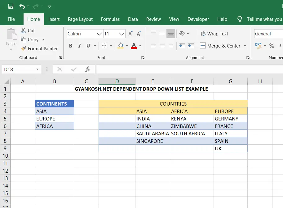
We’ll have the following data.

We have to select a continent and a country.

Three continents are there, EUROPE, ASIA , AFRICA.

The countries in EUROPE are:

GERMANY

FRANCE

ITALY

SPAIN

The countries in ASIA are:

INDIA

CHINA

SAUDI ARABIA

SINGAPORE

The countries in AFRICA are

KENYA

ZIMBABWE

SOUTH AFRICA

We need to select the continent and the next list should only contain the countries in that particular continent to ease up the selection.

As we can see if we use all the names in the single list, we have 12 choices and the user can get confusion in the country and the continent combination. So it is better to give the correct options only. So it is very helpful for the user to get only correct options.

Let us find out the way , we can achieve this.

CREATING SIMPLE LIST FOR CONTINENTS

REFER PICTURE BELOW::

As we have already discussed in detail, the process of creating a simple drop down list.

Look at the picture below in which we have created a simple list for the continents.

Explanation follows the picture.

EXPLANATION

We started with selecting the DATA VALIDATION OPTION from the DATA VALIDATION button under the DATA TAB.
The dialog box opens.
We chose the LIST OPTION from the drop down. The source field activates.
We make the selection of the continent names from the sheet 2, where we have kept all the data.
Click OK.
THE BASIC LIST OF CONTINENTS IS READY.

CREATING A DEPENDENT DROP DOWN LIST IN EXCEL

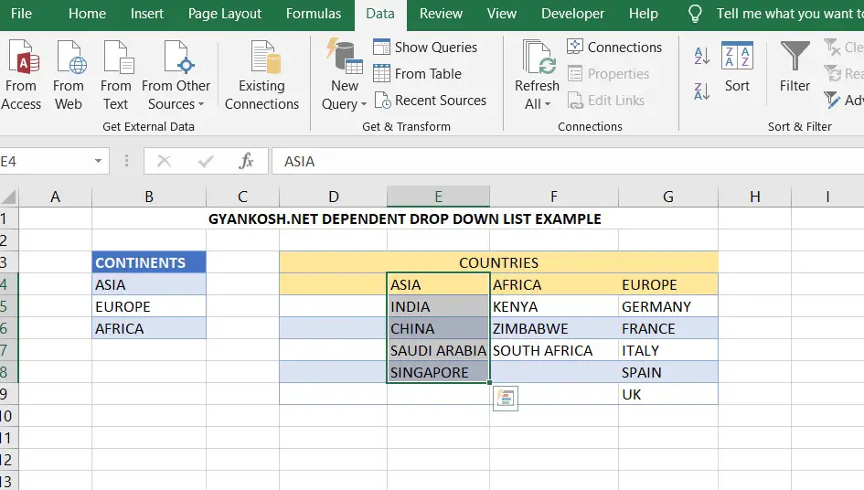
SETTING UP THE DATA

Put the data in different lists so that they are easy to manage.

The data lists can be kept on the same page of the drop down lists, but it is better if we keep them on the other sheet so that we might not mess with them by mistake.

Look at the picture below, how we have organized the data.

NAMING THE DATA RANGE

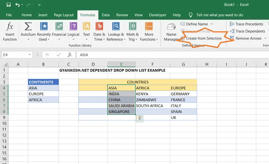
To create the dependent drop down list we need to create THE NAME RANGES of the country lists by the name of the continents. Follow the steps to create ranges with the continent names.

Select the first data range of continent ASIA from the word ASIA TO SINGAPORE i.e. E4:E8 as per our example.(Your range can vary).
Go to FORMULAS tab.

Click CREATE FROM SELECTION.

[This will create the name of the range based on the collection]

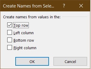
A dialog box will open asking for the basis for the name.
Choose TOP ROW for our case, as we want the name to be based on the heading which is continent name.
Click OK

Now we have successfully named the range as ASIA for all the countries of ASIA continent.
Repeat the process for remaining two ranges too.

The following animation has been given for the reference.

Now all the lists has been named as per the continent names.

Now let us create the list.

ENTERING THE DATA IN THE LIST

Select the cell under the COUNTRIES on the first sheet where we want to populate the list.

Go to DATA VALIDATION under the DATA TAB and choose DATA VALIDATION.

Select LIST from the DROP DOWN.

Refer picture below.

ENTERING THE SOURCE

The whole trick for this all process is the SOURCE of the list.

Now we know that we want the source to be based on the OPTION SELECTED IN THE FIRST LIST.

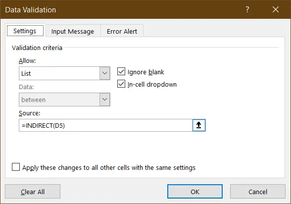
For that we’ll make use of a function named INDIRECT.

INDIRECT FUNCTION RETURNS THE REFERENCE SPECIFIED BY THE TEXT STRING.

It means, suppose we have the text B4 in a cell. Now if we type =Indirect(cell) , it’ll return the value of B4.

For the source here, we’ll use

=INDIRECT(D5), where D5 is the cell containing the chosen continent. Now if we remember, that we have a complete range with that particular range. So that range will get populated into that list.

RUNNING AND CHECKING THE OUTPUT

The following picture shows the running of the example.

We choose the CONTINENT and corresponding COUNTRIES get populated into the list.

We can choose any country from these given choices.

We can see that the example is running as per expectations.

ADDITIONAL CASES FOR SELECTING THE SOURCE FOR THE DEPENDENT LIST

RANGE NAMES HAS SPACES

In the example we just discussed above, we didn’t get this problem of RANGE NAMES as our names were single word. But what if range names are multi words.

When we have space or any other character in between the words and we use the CREATE SELECTION FROM choice to name the range it replaces them with an underscore ” _ “.

e.g.

suppose , if the name of the HEADING is Day of the week, the name will be given as Day_of_the_week

So , there will be a little change the way , we will use our formula in the source.

We’ll make use of a function named SUBSTITUTE here.

SUBSTITUTE function lets us change any character in a text and replace it with another character.

So for this case, we’ll use the formula something like

=INDIRECT( SUBSTITUTE(CELL REFERENCE, ” “,” _”))

Before the text comes to indirect, the name will be changed to the one matching the name of the range by putting an underscore and our problem will be solved.

RANGE NAMES HAS CHARACTERS OTHER THAN A SPACE

Now , we discussed a case where the column names can have a space but what if it has some special character.

Well , in that case too, the SUBSTITUTE FUNCTION would work by just making a small change that we ‘ll change that special character in place of the space.

The following animation shows a complete case of the same.

ANIMATED EXAMPLE

Suppose we talk about the schedule of a school.

We have different actitivities done on different days. Suppose we need to create the details.

Now , it’ll be a great confusion , which activity is done on which day if we need to refer it over and again. So let us solve our problem by creating a dependent list.

We select the day and only the applicable activities populates.

In this example we have the following data.

DAY OF THE WEEK

SUNDAY-MONDAY

TUESDAY-FRIDAY

SATURDAY

ACTIVITIES

SUNDAY-MONDAY	TUESDAY-FRIDAY	SATURDAY
SURFING	WALL CLIMBING	CYCLING
SWIMMING	SKATING	WALKING

So, we create a simple list for the days entries.

Created the ranges of all the Activities by selecting the complete columns as shown in the picture.

We select the cell and start to create a list by going to data validation option under Data tab.

We choose the list and come to the source.

Here, we see that we don’t have space but a hyphen (-).

So we put the following formula in the source

=INDIRECT(SUBSTITUTE(C6,”-“,”_”))

It firstly, substitutes the – with an _ and then feeds the result to the Indirect.

C6 contains the name of the week section i.e. the basic list.

Indirect populates the complete list of activities into the ACTIVITIES COLUMN as per the selection in CHOOSE THE DAY.

The program behaves as per expectations.

Contents